Fiber bundles #
Introduction #
In this section we will approach how to define a general notion of a smooth function on a quiver. To do this we will adapt a construct from continuous mathematics, that of the fiber bundle, to the quiver-geometry setting. Therefore we will briefly review fiber bundles in their traditional form for those that require a refresher, and then explain how to adapt them to quiver geometry.
Continuous fiber bundles #
Motivation #
In continuous geometry, fiber bundles are a kind of gadget to organize and generalize the notion of a continuous function on a topological space.
To motivate why fiber bundles are needed, we will start by looking at three kinds of function: functions on the unit interval, functions on a circle, and "functions on the Möbius strip". The last is in quotations because the story there is a little subtle, and is precisely the kind of situation that fiber bundles can clarify.
First, let \( \fiberSpaceStyle{\topologicalSpace{I_1}} \) denote the half-open interval \( \closedOpenInterval{-1}{1} \sub \re \), and \( \baseSpaceStyle{\topologicalSpace{I_{\piSy}}} \) denote the half-open interval \( \closedOpenInterval{\minus{\piSy}}{\piSy} \sub \re \). Let \( \baseSpaceStyle{\circleSpaceSymbol } \) denote the circle \( \circleSpaceSymbol \sub \realVectorSpace{2} \), seen as the set of points whose distance from the origin is 1:
\[ \baseSpaceStyle{\circleSpaceSymbol }\defEqualSymbol \setConstructor{\TuFo{\baseSpaceElementStyle{\sym{x}}, \baseSpaceElementStyle{\sym{y}}}}{\elemOf{\baseSpaceElementStyle{\sym{x}},\baseSpaceElementStyle{\sym{y}}}{\re},\baseSpaceElementStyle{\sym{x}}^2 + \baseSpaceElementStyle{\sym{y}}^2 = 1} \]We can parameterize \( \baseSpaceStyle{\circleSpaceSymbol } \) in terms of a real number \( \elemOf{\baseSpaceElementStyle{\sym{ \theta }}}{\baseSpaceStyle{\topologicalSpace{I_{\piSy}}}} \) via:
\[ \baseSpaceStyle{\circleSpaceSymbol } = \setConstructor{\TuFo{\sin(\baseSpaceElementStyle{\sym{ \theta }}), \cos(\baseSpaceElementStyle{\sym{ \theta }})}}{\elemOf{\baseSpaceElementStyle{\sym{ \theta }}}{\baseSpaceStyle{\topologicalSpace{I_{\piSy}}}}} \]We will now consider "interval functions" of the form \( \functionType{\baseSpaceStyle{\topologicalSpace{I_{\piSy}}}}{\fiberSpaceStyle{\topologicalSpace{I_1}}} \), and "circle functions" of the form \( \functionType{\baseSpaceStyle{\circleSpaceSymbol }}{\fiberSpaceStyle{\topologicalSpace{I_1}}} \). In other words, these are functions whose domain is the interval \( \baseSpaceStyle{\topologicalSpace{I_{\piSy}}} \) or the circle \( \baseSpaceStyle{\circleSpaceSymbol } \) respectively.
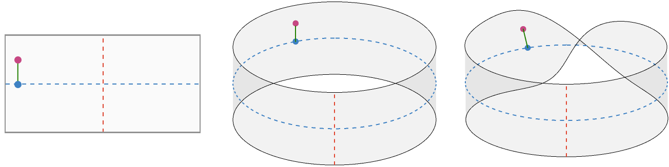
We can visualize these functions via their graphs. For example, here we show two functions: the function \( \functionSignature{\function{\bundleFunctionStyle{\function{f}}}}{\baseSpaceStyle{\topologicalSpace{I_{\piSy}}}}{\fiberSpaceStyle{\topologicalSpace{I_1}}} \) defined by \( \function{\bundleFunctionStyle{\function{f}}}(\baseSpaceElementStyle{\sym{ \theta }}) = \sin(6 \, \baseSpaceElementStyle{\sym{ \theta }}) \), as well as the function \( \functionSignature{\function{\bundleFunctionStyle{\function{\whiteCircleModifier{f}}}}}{\baseSpaceStyle{\circleSpaceSymbol }}{\fiberSpaceStyle{\topologicalSpace{I_1}}} \) defined also as \( \function{\bundleFunctionStyle{\function{\whiteCircleModifier{f}}}}(\baseSpaceElementStyle{\sym{ \theta }}) = \sin(6 \, \baseSpaceElementStyle{\sym{ \theta }}) \), where we use the \( \sym{ \theta } \)-parameterization of \( \baseSpaceStyle{\circleSpaceSymbol } \).
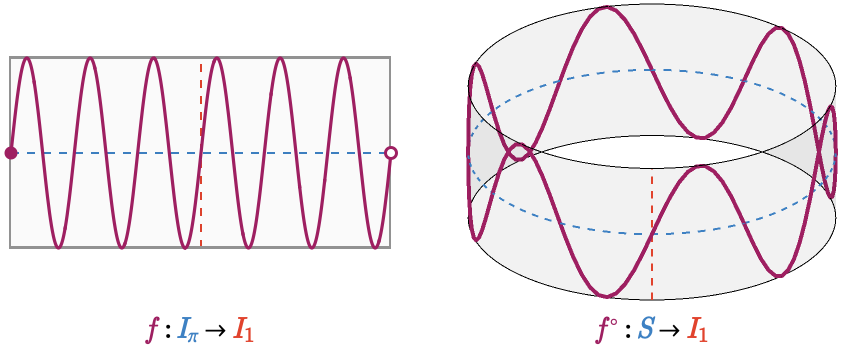
In both cases we have visualized the graph of the function in a space that consists of a "horizontal" subspace representing the domain and an orthogonal "vertical" subspace representing the codomain. For the interval function \( \bundleFunctionStyle{\function{f}} \) the horizontal subspace is 1-dimensional and hence the full graph is a subset of \( \realVectorSpace{2} \). But for the circle function \( \bundleFunctionStyle{\function{\whiteCircleModifier{f}}} \) the horizontal subspace is the circle \( \baseSpaceStyle{\circleSpaceSymbol } \), itself a subset of \( \realVectorSpace{2} \), and hence the full graph is a subset of \( \realVectorSpace{3} \), which is why we plot it as a 3-dimensional figure.
In either case the graph is a subset of a total space that consists of horizontal and vertical subspaces that model the domain and codomain:
-
The graph of the interval function \( \bundleFunctionStyle{\function{f}} \) is the set \( \bundleGraphStyle{\functionGraph{\bundleFunctionStyle{\function{f}}}} = \setConstructor{\TuFo{\baseSpaceElementStyle{\sym{ \theta }}, \function{\bundleFunctionStyle{\function{f}}}(\baseSpaceElementStyle{\sym{ \theta }})}}{\elemOf{\baseSpaceElementStyle{\sym{ \theta }}}{\baseSpaceStyle{\topologicalSpace{I_{\piSy}}}}} \). The graph \( \bundleGraphStyle{\functionGraph{\bundleFunctionStyle{\function{f}}}} \) is a subset \( \bundleGraphStyle{\functionGraph{\bundleFunctionStyle{\function{f}}}} \sub \baseSpaceStyle{\topologicalSpace{I_{\piSy}}}\cartesianProductSymbol \fiberSpaceStyle{\topologicalSpace{I_1}} \) of the total space \( \baseSpaceStyle{\topologicalSpace{I_{\piSy}}}\cartesianProductSymbol \fiberSpaceStyle{\topologicalSpace{I_1}} \).
-
The graph of \( \bundleFunctionStyle{\function{\whiteCircleModifier{f}}} \) is the set \( \bundleGraphStyle{\functionGraph{\bundleFunctionStyle{\function{\whiteCircleModifier{f}}}}} = \setConstructor{\TuFo{\baseSpaceElementStyle{\sym{x}}, \baseSpaceElementStyle{\sym{y}}, \function{\bundleFunctionStyle{\function{\whiteCircleModifier{f}}}}(\TuFo{\baseSpaceElementStyle{\sym{x}}, \baseSpaceElementStyle{\sym{y}}})}}{\elemOf{\TuFo{\baseSpaceElementStyle{\sym{x}}, \baseSpaceElementStyle{\sym{y}}}}{\baseSpaceStyle{\circleSpaceSymbol }}} \). In terms of the \( \sym{ \theta } \)-parameterization, this can be also be written \( \bundleGraphStyle{\functionGraph{\bundleFunctionStyle{\function{\whiteCircleModifier{f}}}}} = \setConstructor{\TuFo{\sin(\baseSpaceElementStyle{\sym{ \theta }}), \cos(\baseSpaceElementStyle{\sym{ \theta }}), \function{\bundleFunctionStyle{\function{f}}}(\baseSpaceElementStyle{\sym{ \theta }})}}{\elemOf{\baseSpaceElementStyle{\sym{ \theta }}}{\baseSpaceStyle{\topologicalSpace{I_{\piSy}}}}} \). The graph \( \bundleGraphStyle{\functionGraph{\bundleFunctionStyle{\function{\whiteCircleModifier{f}}}}} \) is a subset \( \bundleGraphStyle{\functionGraph{\bundleFunctionStyle{\function{\whiteCircleModifier{f}}}}} \sub \baseSpaceStyle{\circleSpaceSymbol }\cartesianProductSymbol \fiberSpaceStyle{\topologicalSpace{I_1}} \) of the total space \( \baseSpaceStyle{\circleSpaceSymbol }\cartesianProductSymbol \fiberSpaceStyle{\topologicalSpace{I_1}} \).
Continuity #
Here we show interval and circle functions defined by \( \sin(\baseSpaceElementStyle{\sym{ \theta }}) \) and \( \sin(\frac{1}{2} \, \baseSpaceElementStyle{\sym{ \theta }}) \).
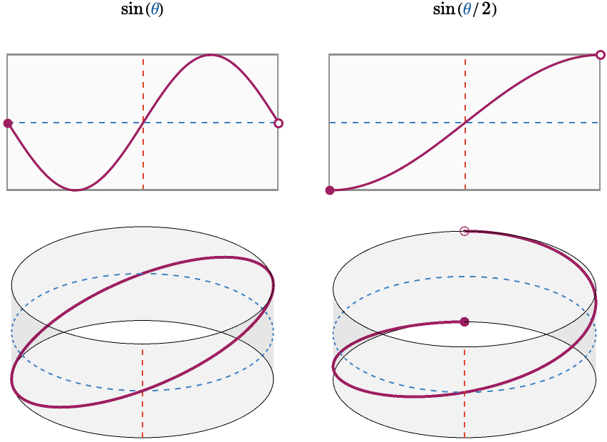
Notice in the top row that both of the interval functions \( \sin(\baseSpaceElementStyle{\sym{ \theta }}) \) and \( \sin(\baseSpaceElementStyle{\sym{ \theta }} / 2) \) appear continuous, as they appear unbroken over the interior of the interval.
In contrast, the circle function \( \sin(\baseSpaceElementStyle{\sym{ \theta }}) \) is continuous, while the circle function \( \sin(\baseSpaceElementStyle{\sym{ \theta }} / 2) \) is not, since it has a break at the far side.
The continuity of these functions can be rephrased as the corresponding graphs being connected, closed sets in the topology of the respective total space: \( \baseSpaceStyle{\topologicalSpace{I_{\piSy}}}\cartesianProductSymbol \fiberSpaceStyle{\topologicalSpace{I_1}} \) for the interval functions, and \( \baseSpaceStyle{\circleSpaceSymbol }\cartesianProductSymbol \fiberSpaceStyle{\topologicalSpace{I_1}} \) for the circle functions. (The real story here is more subtle, but is outside the scope of this treatment). This topological aspect is of fundamental importance for the continuous theory of fiber bundles, but we will not delve into it here, since for discrete fiber bundles topology manifests via the existence of path homomorphisms rather than open and closed sets.
Möbius strip #
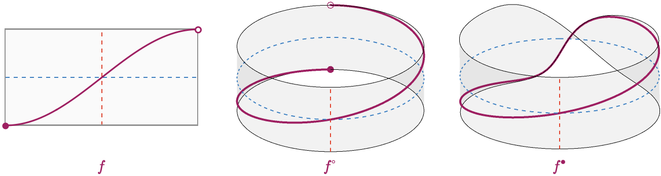
We just saw that the circle function \( \bundleFunctionStyle{\function{\whiteCircleModifier{f}}} \) defined by \( \sin(\baseSpaceElementStyle{\sym{ \theta }} / 2) \) is not continuous. However, if we imagine cutting the band on which the graph of \( \bundleFunctionStyle{\function{\whiteCircleModifier{f}}} \) is shown at the far side, twisting one end of the band, and gluing the ends together again, we will bring the two broken endpoints of the graph into coincidence, joining the break. This is now the graph of some function-like object we'll refer to as \( \bundleFunctionStyle{\function{\blackCircleModifier{f}}} \). Let's visualize this situation:
For functions \( \functionSignature{\function{\bundleFunctionStyle{\function{f}}}}{\baseSpaceStyle{\topologicalSpace{I_{\piSy}}}}{\fiberSpaceStyle{\topologicalSpace{I_1}}} \) that are continuous on \( \baseSpaceStyle{\topologicalSpace{I_{\piSy}}} \), it's not hard to see that if \( \bundleFunctionStyle{\function{f}} \) is even (meaning \( \function{\bundleFunctionStyle{\function{f}}}(\minus{\baseSpaceElementStyle{\sym{x}}}) = \function{\bundleFunctionStyle{\function{f}}}(\baseSpaceElementStyle{\sym{x}}) \)), then \( \bundleFunctionStyle{\function{\whiteCircleModifier{f}}} \) is continuous (on \( \baseSpaceStyle{\circleSpaceSymbol } \)). Likewise if \( \function{f} \) is odd, (meaning \( \function{\bundleFunctionStyle{\function{f}}}(\minus{\baseSpaceElementStyle{\sym{x}}}) = \minus{\function{\bundleFunctionStyle{\function{f}}}(\baseSpaceElementStyle{\sym{x}})} \)), then \( \bundleFunctionStyle{\function{\blackCircleModifier{f}}} \) is continuous (on the "twisted" form of \( \baseSpaceStyle{\circleSpaceSymbol } \)). The only functions that can be continuous on both are those for which \( \function{\bundleFunctionStyle{\function{f}}}(\piSy) = \function{\bundleFunctionStyle{\function{f}}}(\minus{\piSy}) = 0 \) -- where we abuse notation slightly via \( \function{\bundleFunctionStyle{\function{f}}}(\piSy)\syntaxEqualSymbol \limit{\function{\bundleFunctionStyle{\function{f}}}(\baseSpaceElementStyle{\sym{x}})}{\baseSpaceElementStyle{\sym{x}} \to \pi } \).
The band we have created to continuously host the graph of \( \sin(\baseSpaceElementStyle{\sym{ \theta }} / 2) \) is known as the Möbius strip. This is what we hinted at when at the beginning of this section when we said that fiber bundles allow us to define "functions on the Möbius strip". This was of course imprecise language, because \( \bundleFunctionStyle{\function{\blackCircleModifier{f}}} \) itself is defined on the circle, but its "codomain" is somehow a kind of interval that twists around as we move on this circle in a way that is described by the Möbius strip. We cannot think of \( \bundleFunctionStyle{\function{\blackCircleModifier{f}}} \) as being a function of type \( \functionType{\baseSpaceStyle{\circleSpaceSymbol }}{\fiberSpaceStyle{\topologicalSpace{I_1}}} \), since the nature of the interval \( \fiberSpaceStyle{\topologicalSpace{I_1}} \) somehow changes as we proceed around \( \baseSpaceStyle{\circleSpaceSymbol } \) such that it is flipped by the time we complete one revolution around \( \baseSpaceStyle{\circleSpaceSymbol } \).
Conclusion #
We haven't defined any of the machinery of fiber bundles yet, and so this story about the Möbius strip remains informal for now. But hopefully we have motivated a particular approach, which is to think of functions not as maps but as graphs living in some total space that serves as a host, which defines what functions count as continuous. An ordinary function is a graph living in the Cartesian product between the domain and codomain of the function. But there are more general situations for which the total space that hosts the graph of the function is not simply a Cartesian product. It will turn out that we need only that the total space is a Cartesian product locally.
Base, fiber, and total space #
As we saw above, we can think of a function \( \bundleFunctionStyle{\function{f}} \) as a relation between its domain and codomain: this relation is known as the graph \( \bundleGraphStyle{\functionGraph{\bundleFunctionStyle{\function{f}}}} \) of the function. We saw that this graph is a subset of the so-called total space, which in the case of functions on the interval and circle are the Cartesian products \( \baseSpaceStyle{\topologicalSpace{I_{\piSy}}}\cartesianProductSymbol \fiberSpaceStyle{\topologicalSpace{I_1}} \) and \( \baseSpaceStyle{\circleSpaceSymbol }\cartesianProductSymbol \fiberSpaceStyle{\topologicalSpace{I_1}} \). We will now introduce some notation to organize these relationships:
| symbol | name | interval fn's | circle fn's | interpretation |
|---|---|---|---|---|
| \( \baseSpaceStyle{\topologicalSpace{B}} \) | base space | \( \baseSpaceStyle{\topologicalSpace{I_{\piSy}}} \) | \( \baseSpaceStyle{\circleSpaceSymbol } \) | domain; space of inputs |
| \( \totalSpaceStyle{\topologicalSpace{E}} \) | total space | \( \baseSpaceStyle{\topologicalSpace{I_{\piSy}}}\cartesianProductSymbol \fiberSpaceStyle{\topologicalSpace{I_1}} \) | \( \baseSpaceStyle{\circleSpaceSymbol }\cartesianProductSymbol \fiberSpaceStyle{\topologicalSpace{I_1}} \) | host for graph; space of input-output pairs |
| \( \fiberSpaceStyle{\topologicalSpace{F}} \) | fiber space | \( \fiberSpaceStyle{\topologicalSpace{I_1}} \) | \( \fiberSpaceStyle{\topologicalSpace{I_1}} \) | codomain; space of outputs |
The base space \( \baseSpaceStyle{\topologicalSpace{B}} \) plays the role of the domain, the fiber space \( \fiberSpaceStyle{\topologicalSpace{F}} \) plays the role of the codomain, and the total space \( \totalSpaceStyle{\topologicalSpace{E}} \) plays the role of the host for the graph \( \bundleGraphStyle{\functionGraph{\bundleFunctionStyle{\function{f}}}} \) of a function \( \bundleFunctionStyle{\function{f}} \) on the base space: the graph must be an closed, connected subset of the total space with particular properties we will shortly explain.
For the interval and circle functions, the total space is simply the Cartesian product of the base space and the fiber space: \( \totalSpaceStyle{\topologicalSpace{E}} = \baseSpaceStyle{\topologicalSpace{B}}\cartesianProductSymbol \fiberSpaceStyle{\topologicalSpace{F}} \).
Conditions on graphs #
How do we know if a particular (closed, connected) subset \( \bundleGraphStyle{\topologicalSpace{G}} \sub \totalSpaceStyle{\topologicalSpace{E}} \) of the total space \( \totalSpaceStyle{\topologicalSpace{E}} \) corresponds to the graph of some function \( \bundleFunctionStyle{\function{f}} \)? In the special case that the total space can be written as the Cartesian product \( \totalSpaceStyle{\topologicalSpace{E}} = \baseSpaceStyle{\topologicalSpace{B}}\cartesianProductSymbol \fiberSpaceStyle{\topologicalSpace{F}} \), we have the usual conditions for a relation to be a graph: for every point in the base space \( \elemOf{\baseSpaceElementStyle{\sym{x}}}{\baseSpaceStyle{\topologicalSpace{B}}} \) there must be exactly one point in the fiber space \( \elemOf{\fiberSpaceElementStyle{\sym{y}}}{\fiberSpaceStyle{\topologicalSpace{F}}} \) such that \( \elemOf{\TuFo{\baseSpaceElementStyle{\sym{x}}, \fiberSpaceElementStyle{\sym{y}}}}{\bundleGraphStyle{\topologicalSpace{G}}} \). Then \( \bundleGraphStyle{\topologicalSpace{G}} \) is the graph of the function \( \function{\bundleFunctionStyle{\function{f}}}(\baseSpaceElementStyle{\sym{x}}) = \fiberSpaceElementStyle{\sym{y}} \).
For examples, let us consider again the functions \( \functionSignature{\function{\bundleFunctionStyle{\function{f}}}}{\baseSpaceStyle{\topologicalSpace{I_{\piSy}}}}{\fiberSpaceStyle{\topologicalSpace{I_1}}} \) and \( \functionSignature{\function{\bundleFunctionStyle{\function{\whiteCircleModifier{f}}}}}{\baseSpaceStyle{\circleSpaceSymbol }}{\fiberSpaceStyle{\topologicalSpace{I_1}}} \) defined by \( \mto{\baseSpaceElementStyle{\sym{ \theta }}}{\sin(\baseSpaceElementStyle{\sym{ \theta }} / 2)} \):
The graphs of these functions are the relations:
\[ \begin{aligned} \bundleGraphStyle{\functionGraph{\bundleFunctionStyle{\function{f}}}}&= \setConstructor{\TuFo{\baseSpaceElementStyle{\sym{ \theta }}, \sin(\baseSpaceElementStyle{\sym{ \theta }} / 2)}}{\elemOf{\baseSpaceElementStyle{\sym{ \theta }}}{\baseSpaceStyle{\topologicalSpace{I_{\piSy}}}}}\\ \bundleGraphStyle{\functionGraph{\bundleFunctionStyle{\function{\whiteCircleModifier{f}}}}}&= \setConstructor{\TuFo{\sin(\baseSpaceElementStyle{\sym{ \theta }}), \cos(\baseSpaceElementStyle{\sym{ \theta }}), \sin(\baseSpaceElementStyle{\sym{ \theta }} / 2)}}{\elemOf{\baseSpaceElementStyle{\sym{ \theta }}}{\baseSpaceStyle{\topologicalSpace{I_{\piSy}}}}}\end{aligned} \]To write down the graph of \( \bundleFunctionStyle{\function{\blackCircleModifier{f}}} \), we first parameterize the Möbius strip in terms of \( \baseSpaceElementStyle{\sym{ \theta }} \), the angle around the strip, and \( \fiberSpaceElementStyle{\sym{r}} \), the displacement above or below the "equator". We choose an outer radius of 5 and and inner radius of 1, though these are arbitrary:
\[ \function{M}(\baseSpaceElementStyle{\sym{ \theta }},\fiberSpaceElementStyle{\sym{r}})\defEqualSymbol \TuFo{\cos(\baseSpaceElementStyle{\sym{ \theta }}) \, \paren{5 - \fiberSpaceElementStyle{\sym{r}} \, \sin(\baseSpaceElementStyle{\sym{ \theta }} / 2)}, \sin(\baseSpaceElementStyle{\sym{ \theta }}) \, \paren{5 - \fiberSpaceElementStyle{\sym{r}} \, \sin(\baseSpaceElementStyle{\sym{ \theta }} / 2)}, \fiberSpaceElementStyle{\sym{r}} \, \cos(\baseSpaceElementStyle{\sym{ \theta }} / 2)} \]This allows us to define the total space for the strip \( \totalSpaceStyle{\topologicalSpace{M}} \) to be:
\[ \totalSpaceStyle{\topologicalSpace{M}}\defEqualSymbol \setConstructor{\function{M}(\baseSpaceElementStyle{\sym{ \theta }},\fiberSpaceElementStyle{\sym{r}})}{\elemOf{\baseSpaceElementStyle{\sym{ \theta }}}{\baseSpaceStyle{\topologicalSpace{I_{\piSy}}}},\elemOf{\fiberSpaceElementStyle{\sym{r}}}{\fiberSpaceStyle{\topologicalSpace{I_1}}}} \]The graph of \( \bundleFunctionStyle{\function{\blackCircleModifier{f}}} \) is then given by:
\[ \begin{aligned} \bundleGraphStyle{\functionGraph{\bundleFunctionStyle{\function{\blackCircleModifier{f}}}}}&= \setConstructor{\function{M}(\baseSpaceElementStyle{\sym{ \theta }},\sin(\baseSpaceElementStyle{\sym{ \theta }} / 2))}{\elemOf{\baseSpaceElementStyle{\sym{ \theta }}}{\baseSpaceStyle{\topologicalSpace{I_{\piSy}}}}}\\ &= \setConstructor{\TuFo{\cos(\baseSpaceElementStyle{\sym{ \theta }}) \, \paren{9 + \cos(\baseSpaceElementStyle{\sym{ \theta }})}, \sin(\baseSpaceElementStyle{\sym{ \theta }}) \, \paren{9 + \cos(\baseSpaceElementStyle{\sym{ \theta }})}, \sin(\baseSpaceElementStyle{\sym{ \theta }})} / 2}{\elemOf{\baseSpaceElementStyle{\sym{ \theta }}}{\baseSpaceStyle{\topologicalSpace{I_{\piSy}}}}}\end{aligned} \]Projection maps #
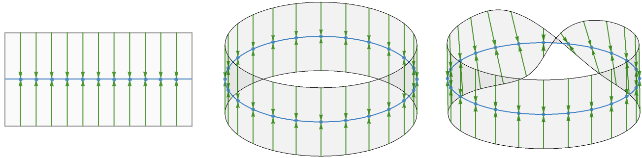
Returning to the question of how we can know when a given subset of \( \totalSpaceStyle{\topologicalSpace{E}} \) could be the graph of some function, we now need to define a projection map \( \functionSignature{\function{\bundleProjectionStyle{\bundleProjection{ \pi }}}}{\totalSpaceStyle{\topologicalSpace{E}}}{\baseSpaceStyle{\topologicalSpace{B}}} \), which is a continuous, surjective function takes us from a point in the total space to the underlying point in the base space. If we think of points in the total space as being input-output pairs, the projection map should send such an input-output pair to its input component. The projection maps for the interval and circle total spaces are therefore the following:
\[ \begin{csarray}{ccccccccc}{acccccccc} \bundleProjectionStyle{\bundleProjection{p}} & : & \baseSpaceStyle{\topologicalSpace{I_{\piSy}}}\cartesianProductSymbol \fiberSpaceStyle{\topologicalSpace{I_1}} & \rarr & \baseSpaceStyle{\topologicalSpace{I_{\piSy}}} & \kern{5pt} & \function{\bundleProjectionStyle{\bundleProjection{p}}}(\baseSpaceElementStyle{\sym{ \theta }},\fiberSpaceElementStyle{\sym{y}}) & ≝ & \baseSpaceElementStyle{\sym{ \theta }}\\ & & & & & & & & \\ \bundleProjectionStyle{\bundleProjection{\whiteCircleModifier{p}}} & : & \baseSpaceStyle{\circleSpaceSymbol }\cartesianProductSymbol \fiberSpaceStyle{\topologicalSpace{I_1}} & \rarr & \baseSpaceStyle{\circleSpaceSymbol } & \kern{5pt} & \function{\bundleProjectionStyle{\bundleProjection{\whiteCircleModifier{p}}}}(\baseSpaceElementStyle{\sym{ \theta }},\fiberSpaceElementStyle{\sym{z}}) & ≝ & \baseSpaceElementStyle{\sym{ \theta }}\\ & & & & & & & & \\ \bundleProjectionStyle{\bundleProjection{\blackCircleModifier{p}}} & : & \totalSpaceStyle{\topologicalSpace{M}} & \rarr & \baseSpaceStyle{\circleSpaceSymbol } & \kern{5pt} & \function{\bundleProjectionStyle{\bundleProjection{\blackCircleModifier{p}}}}(\function{M}(\baseSpaceElementStyle{\sym{ \theta }},\fiberSpaceElementStyle{\sym{r}})) & ≝ & \baseSpaceElementStyle{\sym{ \theta }} \end{csarray} \]For example, here we show a point \( \totalSpaceElementStyle{\sym{e}} = \TuFo{\baseSpaceElementStyle{\sym{ \theta }}, \fiberSpaceElementStyle{\sym{y}}} = \TuFo{-\frac{7}{8} \, \piSy, \frac{1}{2}} \) in the total space and its projection to a point \( \baseSpaceElementStyle{\sym{ \theta }} \) in the base space in all three cases:
We can visualize the action of the projection map as a series of arrows that show how sets of points of the total space \( \totalSpaceStyle{\topologicalSpace{E}} \) are mapped by \( \bundleProjectionStyle{\bundleProjection{ \pi }} \) to points in the base space \( \baseSpaceStyle{\topologicalSpace{B}} \):
We can then rephrase part of the condition that a subset \( \bundleGraphStyle{\topologicalSpace{G}} \sub \totalSpaceStyle{\topologicalSpace{E}} \) of the total space represent a graph. In particular, we can require that the image of the graph be the base space:
\[ \function{\imageModifier{\bundleProjectionStyle{\bundleProjection{ \pi }}}}(\bundleGraphStyle{\topologicalSpace{G}}) = \baseSpaceStyle{\topologicalSpace{B}} \]This ensures that there is at least one element \( \elemOf{\TuFo{\baseSpaceElementStyle{\sym{x}}, \fiberSpaceElementStyle{\sym{y}}}}{\bundleGraphStyle{\topologicalSpace{G}}} \) for every \( \elemOf{\baseSpaceElementStyle{\sym{x}}}{\baseSpaceStyle{\topologicalSpace{B}}} \), in other words, that the function underlying the graph is total.
Now, if there was more than one such pair for a given \( \elemOf{\baseSpaceElementStyle{\sym{x}}}{\baseSpaceStyle{\topologicalSpace{B}}} \), say \( \TuFo{\baseSpaceElementStyle{\sym{x}}, \fiberSpaceElementStyle{\sym{y}}} \) and \( \TuFo{\baseSpaceElementStyle{\sym{x}}, \primed{\fiberSpaceElementStyle{\sym{y}}}} \), then we would effectively have the graph of a multivalued function that takes on a set of values at \( \baseSpaceElementStyle{\sym{x}} \): \( \function{f}(\baseSpaceElementStyle{\sym{x}}) = \SeFo{\fiberSpaceElementStyle{\sym{y}}, \primed{\fiberSpaceElementStyle{\sym{y}}}} \).
To ensure that there is at most one such pair so that we have a single-valued function, we require that there exists a total function \( \functionSignature{\function{\bundleSectionStyle{\bundleSection{ \sigma }}}}{\baseSpaceStyle{\topologicalSpace{B}}}{\totalSpaceStyle{\topologicalSpace{E}}} \) that gives us this single pair for every \( \elemOf{\baseSpaceElementStyle{\sym{x}}}{\baseSpaceStyle{\topologicalSpace{B}}} \).
For example, for our interval function \( \function{\bundleFunctionStyle{\function{f}}}(\baseSpaceElementStyle{\sym{ \theta }}) = \sin(\baseSpaceElementStyle{\sym{ \theta }} / 2) \) the corresponding \( \bundleSectionStyle{\bundleSection{ \sigma }} \) is:
\[ \function{\bundleSectionStyle{\bundleSection{ \sigma }}}(\baseSpaceElementStyle{\sym{ \theta }})\defEqualSymbol \TuFo{\baseSpaceElementStyle{\sym{ \theta }}, \sin(\baseSpaceElementStyle{\sym{ \theta }} / 2)} \]We can visualize the action of \( \bundleFunctionStyle{\function{f}},\bundleFunctionStyle{\function{\whiteCircleModifier{f}}},\bundleFunctionStyle{\function{\blackCircleModifier{f}}} \) as the sets of arrows that show how a point in the base space is mapped to a point in the total space:
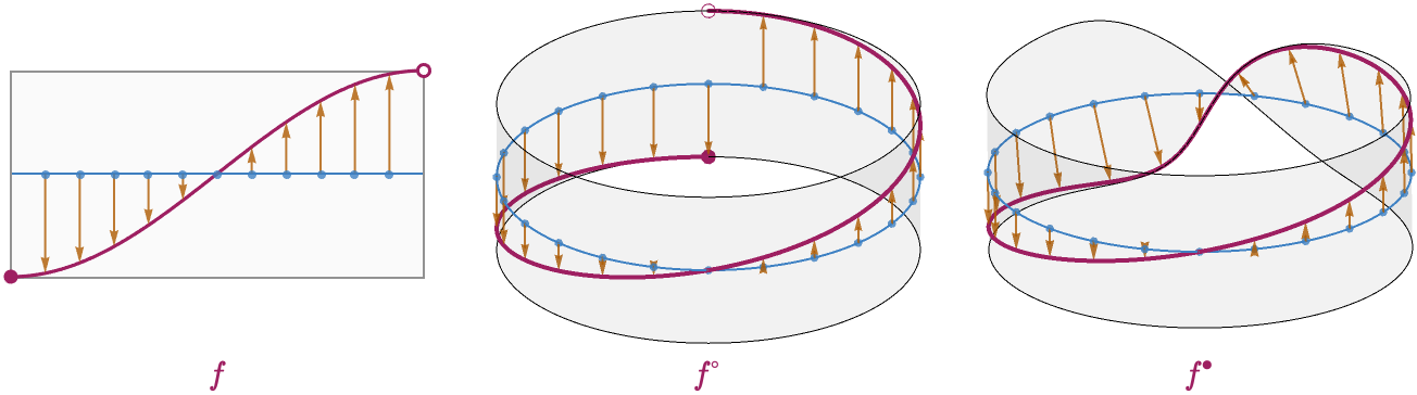
Notice that this function \( \bundleSectionStyle{\bundleSection{ \sigma }} \) must send every \( \elemOf{\baseSpaceElementStyle{\sym{x}}}{\baseSpaceStyle{\topologicalSpace{B}}} \) to a point of \( \totalSpaceStyle{\topologicalSpace{E}} \) that then projects back down to the original point: \( \function{\bundleProjectionStyle{\bundleProjection{ \pi }}}(\function{\bundleSectionStyle{\bundleSection{ \sigma }}}(\baseSpaceElementStyle{\sym{x}}))\identicallyEqualSymbol \baseSpaceElementStyle{\sym{x}} \). Compactly this is the identity:
\[ \functionComposition{\bundleProjectionStyle{\bundleProjection{ \pi }}\functionCompositionSymbol \bundleSectionStyle{\bundleSection{ \sigma }}}\identicallyEqualSymbol \identity_{\baseSpaceStyle{\topologicalSpace{B}}} \]The function \( \bundleSectionStyle{\bundleSection{ \sigma }} \) contains the same information as the graph \( \bundleGraphStyle{\topologicalSpace{G}} \). In fact, the graph is simply the image of the base space under \( \bundleSectionStyle{\bundleSection{ \sigma }} \):
\[ \function{\imageModifier{\bundleSectionStyle{\bundleSection{ \sigma }}}}(\baseSpaceStyle{\topologicalSpace{B}}) = \bundleGraphStyle{\topologicalSpace{G}} \]Summary #
We now have a characterization for when a subset \( \bundleGraphStyle{\topologicalSpace{G}} \) of the total space \( \totalSpaceStyle{\topologicalSpace{E}} \) is the graph of a function-like object on the base space \( \baseSpaceStyle{\topologicalSpace{B}} \):
-
We must first decide on a projection map \( \functionSignature{\function{\bundleProjectionStyle{\bundleProjection{ \pi }}}}{\totalSpaceStyle{\topologicalSpace{E}}}{\baseSpaceStyle{\topologicalSpace{B}}} \) that describes how \( \totalSpaceStyle{\topologicalSpace{E}} \) covers \( \baseSpaceStyle{\topologicalSpace{B}} \), since this determines whether a subset \( \bundleGraphStyle{\topologicalSpace{G}} \sub \totalSpaceStyle{\topologicalSpace{E}} \) corresponds to to the graph of a single-valued function.
-
One this choice is made, a subset \( \bundleGraphStyle{\topologicalSpace{G}} \sub \totalSpaceStyle{\topologicalSpace{E}} \) is the graph of a function-like object if it is the image \( \function{\imageModifier{\bundleSectionStyle{\bundleSection{ \sigma }}}}(\baseSpaceStyle{\topologicalSpace{B}}) = \bundleGraphStyle{\topologicalSpace{G}} \) of \( \baseSpaceStyle{\topologicalSpace{B}} \) under a continuous map \( \functionSignature{\function{\bundleSectionStyle{\bundleSection{ \sigma }}}}{\baseSpaceStyle{\topologicalSpace{B}}}{\totalSpaceStyle{\topologicalSpace{E}}} \), such that \( \functionComposition{\bundleProjectionStyle{\bundleProjection{ \pi }}\functionCompositionSymbol \bundleSectionStyle{\bundleSection{ \sigma }}}\identicallyEqualSymbol \identity_{\baseSpaceStyle{\topologicalSpace{B}}} \).
Sections #
We just explained how a continuous function \( \functionSignature{\function{\bundleSectionStyle{\bundleSection{ \sigma }}}}{\baseSpaceStyle{\topologicalSpace{B}}}{\totalSpaceStyle{\topologicalSpace{E}}} \) satisfying \( \functionComposition{\bundleProjectionStyle{\bundleProjection{ \pi }}\functionCompositionSymbol \bundleSectionStyle{\bundleSection{ \sigma }}}\identicallyEqualSymbol \identity_{\baseSpaceStyle{\topologicalSpace{B}}} \) can be seen as determining the graph of a function-like object \( \bundleGraphStyle{\topologicalSpace{G}} \) on a base space \( \baseSpaceStyle{\topologicalSpace{B}} \), once a projection \( \functionSignature{\function{\bundleProjectionStyle{\bundleProjection{ \pi }}}}{\totalSpaceStyle{\topologicalSpace{E}}}{\baseSpaceStyle{\topologicalSpace{B}}} \) is chosen. To represent and compute with these function-like objects, it turns out to be more convenient to work with \( \bundleSectionStyle{\bundleSection{ \sigma }} \) itself rather than its corresponding graph \( \bundleGraphStyle{\topologicalSpace{G}} \sub \totalSpaceStyle{\topologicalSpace{E}} \).
Such a function \( \functionSignature{\function{\bundleSectionStyle{\bundleSection{ \sigma }}}}{\baseSpaceStyle{\topologicalSpace{B}}}{\totalSpaceStyle{\topologicalSpace{E}}} \) is called a section of the fiber bundle \( \TuFo{\totalSpaceStyle{\topologicalSpace{E}}, \baseSpaceStyle{\topologicalSpace{B}}, \bundleProjectionStyle{\bundleProjection{ \pi }}} \). The fiber bundle encapsulates our choice of where the graphs of functions on \( \baseSpaceStyle{\topologicalSpace{B}} \) should live, sections then represent and encode these graphs.
In the special case that \( \totalSpaceStyle{\topologicalSpace{E}} = \baseSpaceStyle{\topologicalSpace{B}}\cartesianProductSymbol \fiberSpaceStyle{\topologicalSpace{F}} \), which are called trivial fiber bundles, these sections encode the graphs of ordinary functions with domain \( \baseSpaceStyle{\topologicalSpace{B}} \) and codomain \( \fiberSpaceStyle{\topologicalSpace{F}} \). This was the case with our examples \( \bundleFunctionStyle{\function{f}} \) and \( \bundleFunctionStyle{\function{\whiteCircleModifier{f}}} \).
The sections corresponding to the functions \( \bundleFunctionStyle{\function{f}} \) and \( \bundleFunctionStyle{\function{\whiteCircleModifier{f}}} \) are:
\[ \begin{aligned} \function{\bundleSectionStyle{\bundleSection{ \sigma }}}(\baseSpaceElementStyle{\sym{ \theta }})&\defEqualSymbol \TuFo{\baseSpaceElementStyle{\sym{ \theta }}, \sin(\baseSpaceElementStyle{\sym{ \theta }} / 2)}\\[0.75em] \function{\bundleSectionStyle{\bundleSection{\whiteCircleModifier{ \sigma }}}}(\baseSpaceElementStyle{\sym{ \theta }})&\defEqualSymbol \TuFo{\sin(\baseSpaceElementStyle{\sym{ \theta }}), \cos(\baseSpaceElementStyle{\sym{ \theta }}), \sin(\baseSpaceElementStyle{\sym{ \theta }} / 2)}\end{aligned} \]What about the section \( \bundleSectionStyle{\bundleSection{\blackCircleModifier{ \sigma }}} \)? We will explain this in the next... section.
Möbius strip #
The object \( \bundleFunctionStyle{\function{\blackCircleModifier{f}}} \) was a case in which we could not represent the total space as a Cartesian product. For this case, \( \bundleFunctionStyle{\function{\blackCircleModifier{f}}} \) will be a section of a fiber bundle \( \TuFo{\totalSpaceStyle{\topologicalSpace{M}}, \baseSpaceStyle{\circleSpaceSymbol }, \bundleProjectionStyle{\bundleProjection{\blackCircleModifier{p}}}} \), where \( \totalSpaceStyle{\topologicalSpace{M}} \) is the subset of \( \realVectorSpace{3} \) (with its induced topology) that we defined earlier to be:
\[ \begin{aligned} \totalSpaceStyle{\topologicalSpace{M}}&\defEqualSymbol \setConstructor{\function{M}(\baseSpaceElementStyle{\sym{ \theta }},\fiberSpaceElementStyle{\sym{r}})}{\elemOf{\baseSpaceElementStyle{\sym{ \theta }}}{\baseSpaceStyle{\topologicalSpace{I_{\piSy}}}},\elemOf{\fiberSpaceElementStyle{\sym{r}}}{\fiberSpaceStyle{\topologicalSpace{I_1}}}}\\ \function{M}(\baseSpaceElementStyle{\sym{ \theta }},\fiberSpaceElementStyle{\sym{r}})&\defEqualSymbol \TuFo{\cos(\baseSpaceElementStyle{\sym{ \theta }}) \, \paren{5 - \fiberSpaceElementStyle{\sym{r}} \, \sin(\baseSpaceElementStyle{\sym{ \theta }} / 2)}, \sin(\baseSpaceElementStyle{\sym{ \theta }}) \, \paren{5 - \fiberSpaceElementStyle{\sym{r}} \, \sin(\baseSpaceElementStyle{\sym{ \theta }} / 2)}, \fiberSpaceElementStyle{\sym{r}} \, \cos(\baseSpaceElementStyle{\sym{ \theta }} / 2)}\end{aligned} \]The projection \( \functionSignature{\function{\bundleProjectionStyle{\bundleProjection{\blackCircleModifier{p}}}}}{\totalSpaceStyle{\topologicalSpace{M}}}{\baseSpaceStyle{\circleSpaceSymbol }} \) is defined by:
\[ \function{\bundleProjectionStyle{\bundleProjection{\blackCircleModifier{p}}}}(\function{M}(\baseSpaceElementStyle{\sym{ \theta }},\fiberSpaceElementStyle{\sym{r}}))\defEqualSymbol \baseSpaceElementStyle{\sym{ \theta }} \]Then \( \bundleFunctionStyle{\function{\blackCircleModifier{f}}} \) is the function-like object whose graph described by the section:
\[ \function{\bundleSectionStyle{\bundleSection{\blackCircleModifier{ \sigma }}}}(\baseSpaceElementStyle{\sym{ \theta }})\defEqualSymbol \function{M}(\baseSpaceElementStyle{\sym{ \theta }},\sin(\baseSpaceElementStyle{\sym{ \theta }} / 2)) \]Typical fibers and local trivializations #
We saw that the sections \( \bundleSectionStyle{\bundleSection{ \sigma }} \) are generalizations of functions, since they encode graphs of such function-like objects in some total space of the corresponding fiber bundle \( \TuFo{\totalSpaceStyle{\topologicalSpace{E}}, \baseSpaceStyle{\topologicalSpace{B}}, \bundleProjectionStyle{\bundleProjection{ \pi }}} \). For ordinary functions -- which are sections of trivial fiber bundles -- the total space is a Cartesian product \( \totalSpaceStyle{\topologicalSpace{E}} = \baseSpaceStyle{\topologicalSpace{B}}\cartesianProductSymbol \fiberSpaceStyle{\topologicalSpace{F}} \), where the fiber space \( \fiberSpaceStyle{\topologicalSpace{F}} \) plays the role of the codomain of the function. Do we have to completely throw out the notion of such a fiber space for non-trivial fiber bundles? The idea of a codomain seems useful, so we would prefer not to throw the baby out with the bathwater. Luckily, we can still talk about a so-called typical fiber \( \fiberSpaceStyle{\topologicalSpace{F}} \).
The idea is that while the total space may not break down into a straightforward Cartesian product globally, it does break down locally -- meaning that for suitably small open neighborhoods \( \baseSpaceStyle{\topologicalSpace{U}} \sub \baseSpaceStyle{\topologicalSpace{B}} \) of \( \baseSpaceStyle{\topologicalSpace{B}} \) around some point \( \elemOf{\baseSpaceElementStyle{\sym{x}}}{\baseSpaceStyle{\topologicalSpace{B}}} \), we can represent the corresponding portion \( \totalSpaceStyle{\topologicalSpace{V}} \sub \totalSpaceStyle{\topologicalSpace{E}} \) of the total space \( \totalSpaceStyle{\topologicalSpace{E}} \) that lives above \( \baseSpaceStyle{\topologicalSpace{B}} \) as a Cartesian product with the typical fiber \( \fiberSpaceStyle{\topologicalSpace{F}} \):
\[ \begin{aligned} \function{\bundleProjectionStyle{\bundleProjection{ \pi }}}(\totalSpaceStyle{\topologicalSpace{V}} \sub \totalSpaceStyle{\topologicalSpace{E}})&= \baseSpaceStyle{\topologicalSpace{U}} \sub \baseSpaceStyle{\topologicalSpace{B}}\\[0.75em] \totalSpaceStyle{\topologicalSpace{V}}&\homeomorphicSymbol\baseSpaceStyle{\topologicalSpace{U}}\cartesianProductSymbol \fiberSpaceStyle{\topologicalSpace{F}}\end{aligned} \]This is called a local trivialization of \( \totalSpaceStyle{\topologicalSpace{E}} \) around \( \baseSpaceElementStyle{\sym{x}} \). Such a local trivialization is always possible for a fiber bundle (which we will not show here). What makes a non-trivial fiber bundle non-trivial is that we cannot glue together these local trivializations to express the entire total space as such a Cartesian product.
For the interval, circle, and twisted functions we examined above, the typical fiber was in all cases \( \fiberSpaceStyle{\topologicalSpace{F}} = \fiberSpaceStyle{\topologicalSpace{I_1}} \).
Discrete fiber bundles #
How do we recapitulate the setup of continuous fiber bundles for quivers? Let us try the most straightforward approach. We define a quiver fiber bundle to be a tuple \( \TuFo{\totalSpaceStyle{\quiver{E}}, \baseSpaceStyle{\quiver{B}}, \bundleProjectionStyle{\pathHomomorphism{ \pi }}} \), where:
-
\( \totalSpaceStyle{\quiver{E}} \) is the total quiver
-
\( \baseSpaceStyle{\quiver{B}} \) is the base quiver
-
\( \functionSignature{\function{\bundleProjectionStyle{\pathHomomorphism{ \pi }}}}{\totalSpaceStyle{\quiver{E}}}{\baseSpaceStyle{\quiver{B}}} \) is the projection map, a path homomorphism that is moreover a covering map
The special case of a trivial quiver bundle occurs when the total space is a quiver product given by the so-called fiber product:
\[ \totalSpaceStyle{\quiver{E}} = \frac{\quiverProdPoly{\baseSpaceStyle{\forwardFactor }\,\paren{\fiberSpaceStyle{\forwardFactor }+\fiberSpaceStyle{\neutralFactor }+\fiberSpaceStyle{\backwardFactor }}}} {\baseSpaceStyle{\quiver{B}},\fiberSpaceStyle{\quiver{F}}} \]As an example, let us consider a total quiver \( \totalSpaceStyle{\quiver{E}} \) defined to be the fiber product of \( \baseSpaceStyle{\quiver{B}} = \bindCardSize{\subSize{\lineQuiver }{8}}{\card{\daBlFo{b}}} \) and \( \fiberSpaceStyle{\quiver{F}} = \bindCardSize{\subSize{\lineQuiver }{2}}{\card{\daReFo{f}}} \). We show the total space below, alongside its factors:
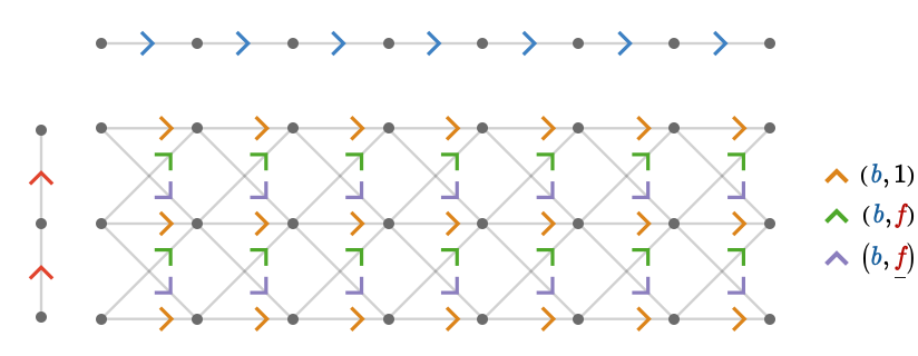
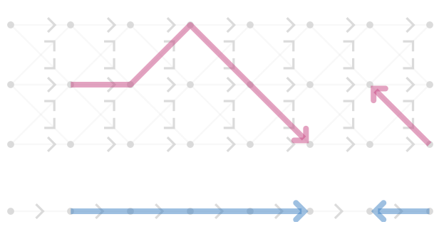
The projection map \( \bundleProjectionStyle{\pathHomomorphism{ \pi }} \) maps a path in the total quiver to the path in the base quiver that consists only of the first factor vertex of each product vertex, and whose cardinals consist of the first factor cardinal of each product cardinal. In other words, the cardinals are mapped as follows:
\[ \assocArray{\mto{\cardinalProduct{\card{\daBlFo{b}},\inverted{\card{\daReFo{f}}}}}{\card{\daBlFo{b}}},\mto{\cardinalProduct{\card{\daBlFo{b}},1}}{\card{\daBlFo{b}}},\mto{\cardinalProduct{\card{\daBlFo{b}},\card{\daReFo{f}}}}{\card{\daBlFo{b}}}} \]Below we visualize the "graph" of a section of this quiver bundle:
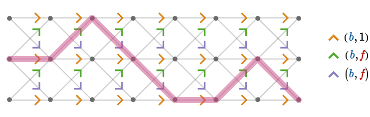
The corresponding section \( \functionSignature{\function{\bundleSectionStyle{\pathHomomorphism{ \sigma }}}}{\baseSpaceStyle{\quiver{B}}}{\totalSpaceStyle{\quiver{E}}} \) is then a path homomorphism that sends a path in the base quiver \( \baseSpaceStyle{\quiver{B}} \) to the corresponding "lifted" path that is a connected component of the fragment of the sub-graph illustrated above. For example, we show the image of two such paths in the base quiver: