Rewriting systems #
Introduction #
We now make our first foray into dynamics: quivers that describe systems that change in time. To do this we will use the lens of rewriting systems. A (computational) rewriting system is a non-deterministic automaton that successively transforms some global state, represented by an arbitrary data structure, by finding and applying well-defined rules that match particular sub-elements of this data structure, replacing them with other elements.
Rewriting systems provide a flexible and general model of computation, and any computational system can be cast into this model: Turing machines, cellular automata, graph rewriting systems, string rewriting systems, register machines, etc. In all cases, these systems can be non-deterministic, although deterministic systems are special cases, which from our point of view will result in rather trivial theories.
Note: this section is only partially complete. The roadmap for this section can be found here.
Local vs global states #
We referred to rewrite systems as involving rewrites that match and replace sub-elements of the data structure representing the full global state. What are these sub-elements? We will approach this idea slowly. For now, we'll suggest that the local states are the smallest possible sub-elements from which a global state can be reconstructed. We'll look at some concrete rewrite systems to build intuition for the behavior of these local states.
Here we show a table indicating reasonable notions of local state for various types of rewriting system:
| system type | global state | local state | |
|---|---|---|---|
| \( \stringRewritingSystem{} \) | string r.s. | string \( \qstring{\character{c}_1 \character{c}_2 \elSy \character{c}_{\sym{n}}} \) | \( \TuFo{\sym{i}, \character{c}_{\sym{i}}} \) |
| \( \circularStringRewritingSystem{} \) | circular string r.s. | circular string \( \qstring{\elSy \character{c}_{\sym{n} - 1} \character{c}_{\sym{n}} \character{c}_1 \character{c}_2 \elSy} \) | \( \TuFo{\sym{i}, \character{c}_{\sym{i}}} \) |
| \( \turingMachineRewritingSystem{} \) | Turing machine | head in state \( \sym{s} \) at cell \( \sym{i} \) on tape \( \qstring{\character{c}_1 \elSy \character{c}_{\sym{n}}} \) | \( \sym{s},\sym{i},\TuFo{\sym{i}, \character{c}_{\sym{i}}} \) |
| \( \cellularAutomatonRewritingSystem{} \) | cellular automaton | vector of cells \( \list{\character{c}_1,\character{c}_2,\elSy,\character{c}_{\sym{n}}} \) | \( \TuFo{\sym{i}, \sym{c}_{\sym{i}}} \) |
| \( \graphRewritingSystem{} \) | graph r.s. | set of edges \( \list{\de{\vert{\sym{t}_1}}{\vert{\sym{h}_1}},\elSy,\de{\vert{\sym{t}_{\sym{n}}}}{\vert{\sym{h}_{\sym{n}}}}} \) | edge \( \de{\vert{\sym{t}_{\sym{i}}}}{\vert{\sym{h}_{\sym{i}}}} \) |
| \( \hypergraphRewritingSystem{} \) | hypergraph r.s. | set of hyperedges \( \list{\sym{e}_1,\sym{e}_2,\elSy,\sym{e}_{\sym{n}}} \) | hyperedge \( \sym{e}_{\sym{i}} \) |
| \( \petriNetRewritingSystem{} \) | Petri net | place occupancy \( \assocArray{\mto{\sym{t}_1}{\sym{N}_1},\elSy,\mto{\sym{t}_{\sym{n}}}{\sym{N}_{\sym{n}}}} \) | \( \TuFo{\sym{t}_{\sym{i}}, \sym{N}_{\sym{i}}} \) |
We will limit our attention initially to string rewriting systems, as these have a simple notion of spatial locality that originates in the linear order of character positions in the string.
Evolution #
Once a particular rewriting system type has been chosen, it remains to specify the rewriting rules that should be applied. We'll indicate the system in a script typeface, typically \( \rewritingSystem{R} \), and list its rules as:
\[ \rewritingSystem{R} = \rewritingRuleBinding{\genericRewritingSystem{}}{\rewritingRule{\sym{L}_1}{\sym{R}_1},\rewritingRule{\sym{L}_2}{\sym{R}_2},\elSy,\rewritingRule{\sym{L}_{\sym{n}}}{\sym{R}_{\sym{n}}}} \]where \( \sym{L}_{\sym{i}} \) is the left-hand-side, or lhs, of the $i^{\textrm{th}}$ rule, and \( \sym{R}_{\sym{i}} \) is the right-hand-side, or rhs.
The lhs specifies a pattern that should match sub-elements of the global state, and the rhs specifies how the matched state should be rewritten to yield a new local state, and hence a new global state. We will also use the word match as a noun, to refer to the sub-elements (the set of local states) that were matched by the rule.
The match can be rewritten, giving us a new global state. Multiple matches can be present in a particular global state: only one of them is rewritten in a particular evolution of the rewriting system. If multiple matches can occur in a given global state, the system is non-deterministic. If a maximum of one match can occur, the system is deterministic.
We will study non-deterministic systems globally, considering all possible evolutions that can occur: we apply all possible matches in a kind of branching process in order to explore their consequences holistically.
After specifying \( \rewritingSystem{R} \), we can now choose an initial state, written \( \sym{s}_0 \). We write the combined data of a rewriting system and an initial state as \( \rewritingStateBinding{\rewritingSystem{R}}{\sym{s}_0} \).
At that point we can evolve the system, which is an iterative process that is carried out either for a fixed number of steps, or alternatively in an ongoing fashion that never terminates. The matches in a particular global state yield successor states of that state. We may sometimes reach a global state that cannot be rewritten because there are no matches: we say that a particular global state has halted.
This process generates a graph, known as a multiway graph or rewrite graph, in which vertices represent global states, and edges represent rewrites. We'll write the process that generates this graph to depth \( \sym{n} \) as:
\[ \multiwayBFS{\rewritingStateBinding{\rewritingSystem{R}}{\sym{s}_0},\sym{n}}\syntaxEqualSymbol \multiwayBFS{\rewritingSystem{R},\sym{s}_0,\sym{n}} \]Computationally, this is a breadth first search that yields a finite a (finite) rewrite graph if it terminates after some finite number of steps. We'll initially avoid defining or reasoning about infinite rewrite graphs.
String rewriting systems #
To illustrate this setup, we'll focus on string rewriting systems, since they are both easy to visualize, familiar to those with experience with computer programming, and fairly easy to analyze.
Our first example will be the following extremely simple system:
\[ \rewritingSystem{R_0}\defEqualSymbol \rewritingRuleBinding{\stringRewritingSystem{}}{\rewritingRule{\lstr{\texttt{b}}}{\lstr{\texttt{a}}}} \]This rewrite system simply replaces the letter \( \lchar{\texttt{b}} \) with the letter \( \lchar{\texttt{a}} \) whereever it occurs.
Here we visualize the rewrite graph generated by \( \multiwayBFS{\rewritingSystem{R_0},\qstring{\lstr{\texttt{bab}}}, \infty } \):
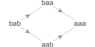
As you can see, there are two matches of the rewrite rule \( \rewritingRule{\lstr{\texttt{b}}}{\lstr{\texttt{a}}} \) in the initial state \( \qstring{\lstr{\texttt{bab}}} \): one corresponding to the character \( \lchar{\texttt{b}} \) occuring in the first string position, the other for the character \( \lchar{\texttt{b}} \) occuring in the third string position. When these matches are rewritten, we obtain two successor global states \( \qstring{\lstr{\texttt{aab}}} \) and \( \qstring{\lstr{\texttt{baa}}} \) respectively. Each of these two global states contain exactly one match, corresponding to the remaining \( \lchar{\texttt{b}} \). Rewriting these, we obtain the same successor global state \( \qstring{\lstr{\texttt{aaa}}} \). This global state contains no matches, as there are no remaining \( \lchar{\texttt{b}} \)'s.
Rewrite quiver #
Notice the important fact here that the two matches, at positions 1 and 3 of the original string, do not overlap: we say that these rewrites commute. This implies that we can rewrite those matches in either order, and the non-rewritten match will still remain. This gives us a hint of how we might attach a cardinal structure to the rewrite graph, yielding the rewrite quiver.
The rewrite quiver is the quiver whose cardinals are the labels formed by the following data taken as a whole: the rule that was matched, and the local states that were involved in the match.
Here we show the rewrite quiver for this simple system, where the two cardinals correspond to the two independent rewrites:
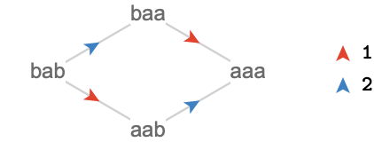
We have named these cardinals with the string position of the match they rewrite, since this is enough to uniquely determine the match for this system.
Let's consider a slightly more complex initial condition of \( \qstring{\lstr{\texttt{bbb}}} \).
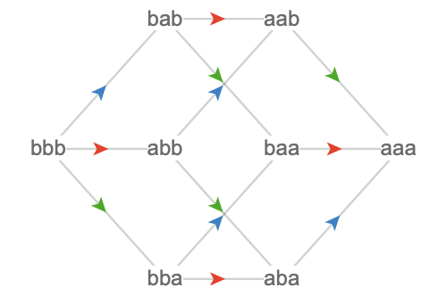
And lastly the initial condition \( \qstring{\lstr{\texttt{bbbb}}} \):
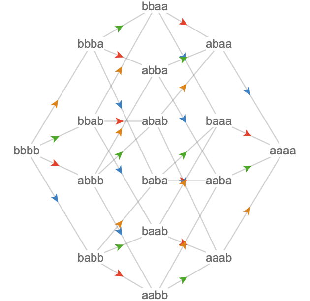
We can see already that this rewrite system yields a rewrite quiver given by \( \subSize{\gridQuiver{\sym{n}}}{2} \), a hypercube of dimension \( \sym{n} \), where \( \sym{n} \) is the count of \( \lchar{\texttt{b}} \)'s in the initial condition. The rewrite quiver is insensitive to the order of the characters in the string, only depending on the \( \lchar{\texttt{b}} \)-count. This is a generic feature of string rewriting systems in which matches do not overlap (whether because of some "cosmic conspiracy" or because the form of the rules prevent this from occurring).
More generally, in any global state of a rewriting system in which we have \( \sym{n} \) commuting rewrites available, we will obtain a subquiver that is isomorphic to \( \subSize{\gridQuiver{\sym{n}}}{2} \).
Sorting system #
We'll now focus on the "sorting system" that partially sorts substrings:
\[ \rewritingSystem{R_1}\defEqualSymbol \rewritingRuleBinding{\stringRewritingSystem{}}{\rewritingRule{\lstr{\texttt{ba}}}{\lstr{\texttt{ab}}}} \]Here we show the rewrite quiver for a variety of initial conditions:
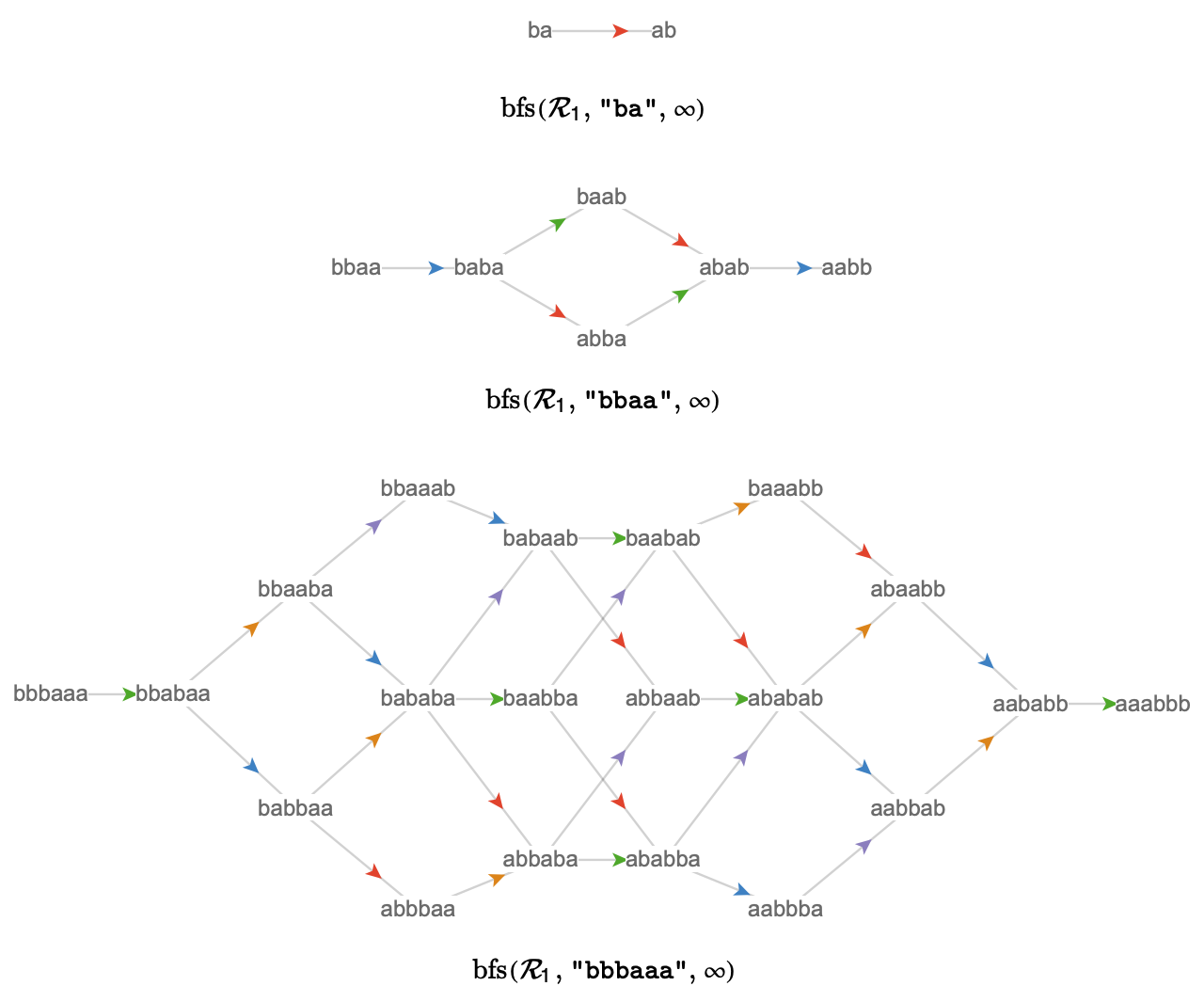
Notice the obvious fact that all of these quivers terminate in a single final state, in which the characters of the string are in sorted order, with all \( \lchar{\texttt{b}} \)'s occurring to the right of all \( \lchar{\texttt{a}} \)'s. This must always happen, since a rewrite always "moves one \( \lchar{\texttt{b}} \) to the right", and will always be able to do so if any \( \lchar{\texttt{a}} \)'s are to the right of any \( \lchar{\texttt{b}} \)'s. The only halting state therefore is the state in which all \( \lchar{\texttt{b}} \)’s are to the right of all \( \lchar{\texttt{a}} \)’s.
Local and global states #
Local and global states #
To ground our discussion, we'll discuss the rewriting system introduced above, initialized to global state \( \lstr{\texttt{bbaa}} \):
\[ \rewritingSystem{R_2}\defEqualSymbol \rewritingStateBinding{\rewritingRuleBinding{\stringRewritingSystem{}}{\rewritingRule{\lstr{\texttt{ba}}}{\lstr{\texttt{ab}}}}}{\lstr{\texttt{bbaa}}} \]This yields the following multiway quiver:
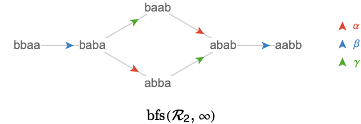
We've already mentioned local states and global states. We'll write the set of local, global states for any initialized rewriting system \( \rewritingSystem{R} \) as \( \localStates{\rewritingSystem{R}} \), \( \globalStates{\rewritingSystem{R}} \), or just \( \localStatesSymbol ,\globalStatesSymbol \) when the rewriting system \( \rewritingSystem{R} \) is fixed. Let's enumerate them for our example \( \rewritingSystem{R_2} \):
\[ \begin{aligned} \globalStates{\rewritingSystem{R_2}}&= \SeFo{\qstring{\lstr{\texttt{bbaa}}}, \qstring{\lstr{\texttt{baba}}}, \qstring{\lstr{\texttt{baab}}}, \qstring{\lstr{\texttt{abba}}}, \qstring{\lstr{\texttt{abab}}}, \qstring{\lstr{\texttt{aabb}}}}\\ \localStates{\rewritingSystem{R_2}}&= \SeFo{\TuFo{1, \lchar{\texttt{a}}}, \TuFo{2, \lchar{\texttt{a}}}, \TuFo{3, \lchar{\texttt{a}}}, \TuFo{4, \lchar{\texttt{a}}}, \TuFo{1, \lchar{\texttt{b}}}, \TuFo{2, \lchar{\texttt{b}}}, \TuFo{3, \lchar{\texttt{b}}}, \TuFo{4, \lchar{\texttt{b}}}}\end{aligned} \]Local key and value substates #
In a string rewriting system, the local states are pairs \( \TuFo{\keySubStateSymbol{p}, \keySubStateSymbol{c}} \) that bind together a string position \( \keySubStateSymbol{p} \) and the character \( \keySubStateSymbol{c} \) that "lives" there. The generic terms we'll use for these are key local substates and value local substates respectively. To explain this terminology: we take the terms key and value from associative array data structures in computer science because a global state cannot contain two local states that share the same key -- this would correspond to characters living at the same string position. We use the term local substate to indicate that these are ingredients of a local state, but they do not individually constitute local states.
The set of key local substates for an initialized rewriting system \( \rewritingSystem{R} \) will be written \( \keySubStates{\rewritingSystem{R}} \), and the set of value local substates will be written \( \valueSubStates{\rewritingSystem{R}} \). Again we'll abbreviate these to \( \keySubStatesSymbol ,\valueSubStatesSymbol \) when \( \rewritingSystem{R} \) is fixed. The set of local substates is then a subset of Cartesian product of these:
\[ \localStatesSymbol \subseteq \keySubStatesSymbol \cartesianProductSymbol \valueSubStatesSymbol \]To be more concise we'll also sometimes write a local substate \( \TuFo{\keySubStateSymbol{p}, \keySubStateSymbol{c}} \) as \( \localState{\keySubStateSymbol{p}}{\keySubStateSymbol{c}} \). Using this notation, the set of local states for \( \rewritingSystem{R_2} \) is:
\[ \localStates{\rewritingSystem{R_2}} = \SeFo{\localState{1}{\lchar{\texttt{a}}}, \localState{2}{\lchar{\texttt{a}}}, \localState{3}{\lchar{\texttt{a}}}, \localState{4}{\lchar{\texttt{a}}}, \localState{1}{\lchar{\texttt{b}}}, \localState{2}{\lchar{\texttt{b}}}, \localState{3}{\lchar{\texttt{b}}}, \localState{4}{\lchar{\texttt{b}}}} \]We have \( \localStatesSymbol \subseteq \keySubStatesSymbol \cartesianProductSymbol \valueSubStatesSymbol \) rather than \( \localStatesSymbol = \keySubStatesSymbol \cartesianProductSymbol \valueSubStatesSymbol \) because, for a given initialized rewriting system, rewriting might not produce all of the theoretically possible local states. For example, the system \( \rewritingSystem{R} = \rewritingStateBinding{\rewritingRuleBinding{\stringRewritingSystem{}}{\rewritingRule{\lstr{\texttt{b}}}{\lstr{\texttt{a}}}}}{\qstring{\lstr{\texttt{aab}}}} \) never creates the local state \( \localState{1}{\lchar{\texttt{b}}} \). The set of local states is actually \( \localStates{\rewritingSystem{R}} = \SeFo{\localState{1}{\lchar{\texttt{a}}}, \localState{2}{\lchar{\texttt{a}}}, \localState{3}{\lchar{\texttt{a}}}, \localState{3}{\lchar{\texttt{b}}}} \).
For the main example \( \rewritingSystem{R_2} \), we happen to have that every possible local state is generated by the system:
\[ \begin{aligned} \keySubStates{\rewritingSystem{R_2}}&= \SeFo{1, 2, 3, 4}\\ \valueSubStates{\rewritingSystem{R_2}}&= \SeFo{\lchar{\texttt{a}}, \lchar{\texttt{b}}}\\[0.75em] \localStates{\rewritingSystem{R_2}}&= \keySubStates{\rewritingSystem{R_2}}\cartesianProductSymbol \valueSubStates{\rewritingSystem{R_2}}\\ &= \SeFo{\localState{1}{\lchar{\texttt{a}}}, \localState{2}{\lchar{\texttt{a}}}, \localState{3}{\lchar{\texttt{a}}}, \localState{4}{\lchar{\texttt{a}}}, \localState{1}{\lchar{\texttt{b}}}, \localState{2}{\lchar{\texttt{b}}}, \localState{3}{\lchar{\texttt{b}}}, \localState{4}{\lchar{\texttt{b}}}}\end{aligned} \]Key substates and length-preserving systems #
In the definitions above, we have implicitly relied the fact the rewrites in the system \( \rewritingSystem{R_2} = \rewritingRuleBinding{\stringRewritingSystem{}}{\rewritingRule{\lstr{\texttt{ba}}}{\lstr{\texttt{ab}}}} \) do not change the length of the string. That is to say, the length of the lhs and rhs are equal, both being 2. This allows us to unambiguously talk of global string positions, and making the set \( \keySubStates{\rewritingSystem{R_2}} = \SeFo{1, 2, 3, 4} \) well defined.
For a rewriting system like \( \rewritingRuleBinding{\stringRewritingSystem{}}{\rewritingRule{\lstr{\texttt{ab}}}{\lstr{\texttt{a}}}} \), however, rewrites will change the length of the string. We might regard such rewrites as effectively removing key substates, making them inaccessible from all rewrites that follow. Conversely, systems like \( \rewritingRuleBinding{\stringRewritingSystem{}}{\rewritingRule{\lstr{\texttt{a}}}{\lstr{\texttt{ab}}}} \) effectively introduce new key substates. To handle such cases, we can expect to define equivalence classes that capture when two local states involving different key substates are actually the same from the point of view of a global or regional state.
There is a host of subtle issues hiding here, and so we will postpone considering such systems for now.
Regional states #
We can see local and global states as living at either end of a continuum of specificity: local states are the "minimal units" of information we have about the state of a rewrite system, whereas global states are maximal in that same sense.
This continuum contains other kinds of states, which are intermediate in the amount of information they contain about the state of the rewrite system. We'll call these regional states. One way to approach conceptualize regional states is by building them up from local states. More precisely, we can think of a regional state as being a set of compatible local states, meaning a set of local states in which there is only one element with any given key substate. In the case of string rewrite systems, compatibility amounts to saying that only one character can live at a given position of a string.
Notation #
We’ll write a regional state consisting of \( \sym{n} \) local states \( \localStateSymbol{l_{\sym{i}}} \) as \( \regionalStateForm{\localStateSymbol{l_1} \localStateSymbol{l_2} \elSy \localStateSymbol{l_{\sym{n}}}} \), and the set of all regional states of a system \( \rewritingSystem{R} \) as \( \regionalStates{\rewritingSystem{R}} \), abbreviating to \( \regionalStatesSymbol \) when \( \rewritingSystem{R} \) is fixed.
A regional state is a partial description of a global state. For string rewriting systems, in which global states are strings, a regional state is then a partial description of a string, which defines that certain string positions have certain character values, but can leave other parts of the string unspecified. We can therefore use wildcard notation to evoke this interpretation, where a dash to indicates a wildcard -- a position in the string for what the regional state does not specify a character value.
Here we show some string regional states written in parentheses notation as well as wildcard notation:
\[ \begin{aligned} \regionalStateForm{\localState{1}{\lchar{\texttt{a}}} \localState{2}{\lchar{\texttt{b}}} \localState{3}{\lchar{\texttt{a}}} \localState{4}{\lchar{\texttt{b}}}}&\syntaxEqualSymbol \wstring{\lstr{\texttt{abab}}}\\ \regionalStateForm{\localState{1}{\lchar{\texttt{a}}} \localState{2}{\lchar{\texttt{b}}} \localState{4}{\lchar{\texttt{b}}}}&\syntaxEqualSymbol \wstring{\lstr{\texttt{ab-b}}}\\ \regionalStateForm{\localState{1}{\lchar{\texttt{a}}}}&\syntaxEqualSymbol \wstring{\lstr{\texttt{a---}}}\\ \regionalStateForm{\localState{4}{\lchar{\texttt{b}}}}&\syntaxEqualSymbol \wstring{\lstr{\texttt{---b}}}\\ \emptyRegionalState &\syntaxEqualSymbol \wstring{\lstr{\texttt{----}}}\end{aligned} \]Gluing #
We can form a regional states by gluing a set of local states. We’ll write this function explicitly as \( \stateCompose \), or an infix form as \( \infixStateComposeSymbol \). This gluing function has the following signature:
\[ \partialFunctionSignature{\stateCompose}{\powerSet{\localStatesSymbol }}{\regionalStatesSymbol } \]Note the symbol \( \rightharpoonup \), which indicates that \( \stateCompose \) is a partial function, not necessarily defined on all sets of local states. This is due to the fact that we cannot glue incompatible local states: local states that share a key substate but differ in their value substate -- we cannot have more than one distinct character at a given string position. We indicate this with notation \( \stateCompose(\elSy) = \invalidRegionalState \).
Examples #
Here we give some examples of gluing operations and their results, both in parentheses and wildcard notation:
\[ \begin{csarray}{rllllll}{acccccc} & & \stateCompose(\SeFo{}) & = & \wstring{\lstr{\texttt{----}}} & \syntaxEqualSymbol & \emptyRegionalState \\ & & \stateCompose(\SeFo{\localState{1}{\lchar{\texttt{a}}}}) & = & \wstring{\lstr{\texttt{a---}}} & \syntaxEqualSymbol & \regionalStateForm{\localState{1}{\lchar{\texttt{a}}}}\\ \localState{1}{\lchar{\texttt{a}}}\infixStateComposeSymbol \localState{2}{\lchar{\texttt{b}}} & \syntaxEqualSymbol & \stateCompose(\SeFo{\localState{1}{\lchar{\texttt{a}}}, \localState{2}{\lchar{\texttt{b}}}}) & = & \wstring{\lstr{\texttt{ab--}}} & \syntaxEqualSymbol & \regionalStateForm{\localState{1}{\lchar{\texttt{a}}} \localState{2}{\lchar{\texttt{b}}}}\\ \localState{1}{\lchar{\texttt{a}}}\infixStateComposeSymbol \localState{2}{\lchar{\texttt{b}}}\infixStateComposeSymbol \localState{4}{\lchar{\texttt{b}}} & \syntaxEqualSymbol & \stateCompose(\SeFo{\localState{1}{\lchar{\texttt{a}}}, \localState{2}{\lchar{\texttt{b}}}, \localState{4}{\lchar{\texttt{b}}}}) & = & \wstring{\lstr{\texttt{ab-b}}} & \syntaxEqualSymbol & \regionalStateForm{\localState{1}{\lchar{\texttt{a}}} \localState{2}{\lchar{\texttt{b}}} \localState{4}{\lchar{\texttt{b}}}}\\ \localState{1}{\lchar{\texttt{a}}}\infixStateComposeSymbol \localState{2}{\lchar{\texttt{b}}}\infixStateComposeSymbol \localState{3}{\lchar{\texttt{b}}}\infixStateComposeSymbol \localState{4}{\lchar{\texttt{a}}} & \syntaxEqualSymbol & \stateCompose(\SeFo{\localState{1}{\lchar{\texttt{a}}}, \localState{2}{\lchar{\texttt{b}}}, \localState{3}{\lchar{\texttt{b}}}, \localState{4}{\lchar{\texttt{a}}}}) & = & \wstring{\lstr{\texttt{abba}}} & \syntaxEqualSymbol & \regionalStateForm{\localState{1}{\lchar{\texttt{a}}} \localState{2}{\lchar{\texttt{b}}} \localState{3}{\lchar{\texttt{b}}} \localState{4}{\lchar{\texttt{a}}}} \end{csarray} \]Melting #
The inverse to gluing is melting, in which we dissolve the glue, obtaining the set of local states that form a particular regional state. The function that melts a regional state into a set of local states is written \( \stateDecompose \), and has the following signature:
\[ \functionSignature{\stateDecompose}{\regionalStatesSymbol }{\powerSet{\localStatesSymbol }} \]We show some obvious examples:
\[ \begin{aligned} \stateDecompose(\wstring{\lstr{\texttt{----}}})&= \SeFo{}\\ \stateDecompose(\wstring{\lstr{\texttt{a---}}})&= \SeFo{\localState{1}{\lchar{\texttt{a}}}}\\ \stateDecompose(\wstring{\lstr{\texttt{ab--}}})&= \SeFo{\localState{1}{\lchar{\texttt{a}}}, \localState{2}{\lchar{\texttt{b}}}}\\ \stateDecompose(\wstring{\lstr{\texttt{ab-b}}})&= \SeFo{\localState{1}{\lchar{\texttt{a}}}, \localState{2}{\lchar{\texttt{b}}}, \localState{4}{\lchar{\texttt{b}}}}\\ \stateDecompose(\wstring{\lstr{\texttt{abba}}})&= \SeFo{\localState{1}{\lchar{\texttt{a}}}, \localState{2}{\lchar{\texttt{b}}}, \localState{3}{\lchar{\texttt{b}}}, \localState{4}{\lchar{\texttt{a}}}}\end{aligned} \]Gluing the melt of a regional state yields that regional state:
\[ \forAllForm{\elemOf{\regionalStateSymbol{R}}{\regionalStatesSymbol }}{\stateCompose(\stateDecompose(\regionalStateSymbol{R})) = \regionalStateSymbol{R}} \]Melting the glue of a set of compatible local states yields that set:
\[ \forAllForm{\elemOf{\setSymbol{S}}{\powerSet{\localStatesSymbol }},\stateCompose(\setSymbol{S}) \neq \invalidRegionalState }{\stateDecompose(\stateCompose(\regionalStateSymbol{S})) = \setSymbol{S}} \]Identifying global and local states with regional states #
We can identify global states of \( \rewritingSystem{R} \), shown on the left, with "maximal" regional states, shown on the right, first in parentheses and then wildcard notation:
\[ \begin{aligned} \qstring{\lstr{\texttt{aabb}}}& \approx \regionalStateForm{\localState{1}{\lchar{\texttt{a}}} \localState{2}{\lchar{\texttt{a}}} \localState{3}{\lchar{\texttt{b}}} \localState{4}{\lchar{\texttt{b}}}}\syntaxEqualSymbol \wstring{\lstr{\texttt{aabb}}}\\ \qstring{\lstr{\texttt{abab}}}& \approx \regionalStateForm{\localState{1}{\lchar{\texttt{a}}} \localState{2}{\lchar{\texttt{b}}} \localState{3}{\lchar{\texttt{a}}} \localState{4}{\lchar{\texttt{b}}}}\syntaxEqualSymbol \wstring{\lstr{\texttt{abab}}}\\ \qstring{\lstr{\texttt{abba}}}& \approx \regionalStateForm{\localState{1}{\lchar{\texttt{a}}} \localState{2}{\lchar{\texttt{b}}} \localState{3}{\lchar{\texttt{b}}} \localState{4}{\lchar{\texttt{a}}}}\syntaxEqualSymbol \wstring{\lstr{\texttt{abba}}}\\ \qstring{\lstr{\texttt{baab}}}& \approx \regionalStateForm{\localState{1}{\lchar{\texttt{b}}} \localState{2}{\lchar{\texttt{a}}} \localState{3}{\lchar{\texttt{a}}} \localState{4}{\lchar{\texttt{b}}}}\syntaxEqualSymbol \wstring{\lstr{\texttt{baab}}}\\ \qstring{\lstr{\texttt{baba}}}& \approx \regionalStateForm{\localState{1}{\lchar{\texttt{b}}} \localState{2}{\lchar{\texttt{a}}} \localState{3}{\lchar{\texttt{b}}} \localState{4}{\lchar{\texttt{a}}}}\syntaxEqualSymbol \wstring{\lstr{\texttt{baba}}}\\ \qstring{\lstr{\texttt{bbaa}}}& \approx \regionalStateForm{\localState{1}{\lchar{\texttt{b}}} \localState{2}{\lchar{\texttt{b}}} \localState{3}{\lchar{\texttt{a}}} \localState{4}{\lchar{\texttt{a}}}}\syntaxEqualSymbol \wstring{\lstr{\texttt{bbaa}}}\end{aligned} \]Note that there are no wildcards actually present in the right hand column, since global states imply a character value for every string position.
Similarly we can identify local states, shown on the left, with "minimal" regional states, shown on the right in set and then wildcard notation:
\[ \begin{csarray}{rclrcl}{aeeiee} \localState{1}{\lchar{\texttt{a}}} & \approx & \regionalStateForm{\localState{1}{\lchar{\texttt{a}}}}\syntaxEqualSymbol \wstring{\lstr{\texttt{a---}}} & \localState{1}{\lchar{\texttt{b}}} & \approx & \regionalStateForm{\localState{1}{\lchar{\texttt{b}}}}\syntaxEqualSymbol \wstring{\lstr{\texttt{b---}}}\\ \localState{2}{\lchar{\texttt{a}}} & \approx & \regionalStateForm{\localState{2}{\lchar{\texttt{a}}}}\syntaxEqualSymbol \wstring{\lstr{\texttt{-a--}}} & \localState{2}{\lchar{\texttt{b}}} & \approx & \regionalStateForm{\localState{2}{\lchar{\texttt{b}}}}\syntaxEqualSymbol \wstring{\lstr{\texttt{-b--}}}\\ \localState{3}{\lchar{\texttt{a}}} & \approx & \regionalStateForm{\localState{3}{\lchar{\texttt{a}}}}\syntaxEqualSymbol \wstring{\lstr{\texttt{--a-}}} & \localState{3}{\lchar{\texttt{b}}} & \approx & \regionalStateForm{\localState{3}{\lchar{\texttt{b}}}}\syntaxEqualSymbol \wstring{\lstr{\texttt{--b-}}}\\ \localState{4}{\lchar{\texttt{a}}} & \approx & \regionalStateForm{\localState{4}{\lchar{\texttt{a}}}}\syntaxEqualSymbol \wstring{\lstr{\texttt{---a}}} & \localState{4}{\lchar{\texttt{b}}} & \approx & \regionalStateForm{\localState{4}{\lchar{\texttt{b}}}}\syntaxEqualSymbol \wstring{\lstr{\texttt{---b}}} \end{csarray} \]We'll denote both the functions that embed global and local states into the regional states with \( \function{ \iota } \):
\[ \begin{nsarray}{c} \functionSignature{\function{ \iota }}{\localStatesSymbol }{\regionalStatesSymbol }\\ \functionSignature{\function{ \iota }}{\globalStatesSymbol }{\regionalStatesSymbol } \end{nsarray} \]Conjunctions #
It is possible to lift the idea of gluing up a level, obtaining an operation we'll call conjunction. Gluing applies to sets of local states; conjunction applies to sets of regional states. We'll write conjunction as \( \stateJoin \) or in infix form as \( \infixStateJoinSymbol \). Conjunction has the following signature:
\[ \partialFunctionSignature{\stateJoin}{\powerSet{\regionalStatesSymbol }}{\regionalStatesSymbol } \]Conjunction of two regional states can be defined in terms of their underlying local states: we form the conjunction by gluing the union of their melts:
\[ \regionalStateSymbol{R}\infixStateJoinSymbol \regionalStateSymbol{S}\defEqualSymbol \stateCompose(\stateDecompose(\regionalStateSymbol{R})\setUnionSymbol \stateDecompose(\regionalStateSymbol{S})) \]This operation can clearly fail when there is a local state in one regional state that is incompatible with a local state in the other regional state, hence \( \stateJoin \) is a partial function.
Here are some examples of conjunction on regional states:
\[ \begin{csarray}{ccccc}{acccc} \emptyRegionalState & \sqcup & \emptyRegionalState & = & \emptyRegionalState \\ \regionalStateForm{\localState{1}{\lchar{\texttt{b}}}} & \sqcup & \emptyRegionalState & = & \regionalStateForm{\localState{1}{\lchar{\texttt{b}}}}\\ \regionalStateForm{\localState{1}{\lchar{\texttt{b}}}} & \sqcup & \regionalStateForm{\localState{1}{\lchar{\texttt{a}}}} & = & \invalidRegionalState \\ \regionalStateForm{\localState{1}{\lchar{\texttt{b}}}} & \sqcup & \regionalStateForm{\localState{2}{\lchar{\texttt{a}}}} & = & \regionalStateForm{\localState{1}{\lchar{\texttt{b}}} \localState{2}{\lchar{\texttt{a}}}}\\ \regionalStateForm{\localState{1}{\lchar{\texttt{a}}} \localState{2}{\lchar{\texttt{b}}} \localState{3}{\lchar{\texttt{a}}}} & \sqcup & \regionalStateForm{\localState{2}{\lchar{\texttt{b}}} \localState{3}{\lchar{\texttt{a}}} \localState{4}{\lchar{\texttt{b}}}} & = & \regionalStateForm{\localState{1}{\lchar{\texttt{a}}} \localState{2}{\lchar{\texttt{b}}} \localState{3}{\lchar{\texttt{a}}} \localState{4}{\lchar{\texttt{b}}}}\\ \regionalStateForm{\localState{1}{\lchar{\texttt{a}}} \localState{2}{\lchar{\texttt{b}}}} & \sqcup & \regionalStateForm{\localState{3}{\lchar{\texttt{a}}} \localState{4}{\lchar{\texttt{b}}}} & = & \regionalStateForm{\localState{1}{\lchar{\texttt{a}}} \localState{2}{\lchar{\texttt{b}}} \localState{3}{\lchar{\texttt{a}}} \localState{4}{\lchar{\texttt{b}}}}\\ \regionalStateForm{\localState{1}{\lchar{\texttt{a}}} \localState{2}{\lchar{\texttt{a}}} \localState{3}{\lchar{\texttt{a}}}} & \sqcup & \regionalStateForm{\localState{2}{\lchar{\texttt{b}}} \localState{3}{\lchar{\texttt{b}}} \localState{4}{\lchar{\texttt{b}}}} & = & \invalidRegionalState \end{csarray} \]We can also depict these same examples with wildcard notation, with the conjunction appearing under its operands:
\[ \begin{array}{cccccccc} \regionalStateSymbol{R} & \wstring{\lstr{\texttt{----}}} & \wstring{\lstr{\texttt{b---}}} & \wstring{\lstr{\texttt{b---}}} & \wstring{\lstr{\texttt{b---}}} & \wstring{\lstr{\texttt{aba-}}} & \wstring{\lstr{\texttt{ab--}}} & \wstring{\lstr{\texttt{aaa-}}}\\[1em] \regionalStateSymbol{S} & \wstring{\lstr{\texttt{----}}} & \wstring{\lstr{\texttt{----}}} & \wstring{\lstr{\texttt{a---}}} & \wstring{\lstr{\texttt{-a--}}} & \wstring{\lstr{\texttt{-bab}}} & \wstring{\lstr{\texttt{--ab}}} & \wstring{\lstr{\texttt{-bbb}}}\\[1em] \regionalStateSymbol{R}\infixStateJoinSymbol \regionalStateSymbol{S} & \wstring{\lstr{\texttt{----}}} & \wstring{\lstr{\texttt{b---}}} & \invalidRegionalState & \wstring{\lstr{\texttt{ba--}}} & \wstring{\lstr{\texttt{abab}}} & \wstring{\lstr{\texttt{abab}}} & \invalidRegionalState \end{array} \]Disjunctions #
Similar to the operation of conjunction, we can define disjunction, which finds the regional state that is in common to two or more input regional states. We'll write the disjunction function as \( \stateMeet \), and in infix form as \( \infixStateMeetSymbol \). Disjunction has the following signature:
\[ \functionSignature{\stateMeet}{\powerSet{\regionalStatesSymbol }}{\regionalStatesSymbol } \]Unlike conjunction, disjunction is a total function: it is defined on every set of regional states. We can define the disjunction of two regional states in terms of \( \stateDecompose \) and \( \stateCompose \) as follows:
\[ \regionalStateSymbol{R}\infixStateMeetSymbol \regionalStateSymbol{S}\defEqualSymbol \stateCompose(\stateDecompose(\regionalStateSymbol{R})\setIntersectionSymbol \stateDecompose(\regionalStateSymbol{S})) \]The totality of \( \stateMeet \) is a consequence of the fact that the local states in the melt of \( \regionalStateSymbol{R} \) are, by definition, compatible, and likewise for \( \regionalStateSymbol{S} \). Hence the local states in their intersection must be compatible too.
\[ \begin{csarray}{ccccc}{acccc} \emptyRegionalState & \sqcap & \emptyRegionalState & = & \emptyRegionalState \\ \regionalStateForm{\localState{1}{\lchar{\texttt{b}}}} & \sqcap & \emptyRegionalState & = & \emptyRegionalState \\ \regionalStateForm{\localState{1}{\lchar{\texttt{b}}}} & \sqcap & \regionalStateForm{\localState{1}{\lchar{\texttt{a}}}} & = & \emptyRegionalState \\ \regionalStateForm{\localState{1}{\lchar{\texttt{b}}}} & \sqcap & \regionalStateForm{\localState{1}{\lchar{\texttt{b}}} \localState{2}{\lchar{\texttt{b}}}} & = & \regionalStateForm{\localState{1}{\lchar{\texttt{b}}}}\\ \regionalStateForm{\localState{1}{\lchar{\texttt{a}}} \localState{2}{\lchar{\texttt{a}}} \localState{3}{\lchar{\texttt{a}}}} & \sqcap & \regionalStateForm{\localState{2}{\lchar{\texttt{a}}} \localState{3}{\lchar{\texttt{a}}} \localState{4}{\lchar{\texttt{a}}}} & = & \regionalStateForm{\localState{2}{\lchar{\texttt{a}}} \localState{3}{\lchar{\texttt{a}}}}\\ \regionalStateForm{\localState{1}{\lchar{\texttt{a}}} \localState{2}{\lchar{\texttt{a}}} \localState{3}{\lchar{\texttt{a}}} \localState{4}{\lchar{\texttt{a}}}} & \sqcap & \regionalStateForm{\localState{1}{\lchar{\texttt{b}}} \localState{2}{\lchar{\texttt{a}}} \localState{3}{\lchar{\texttt{a}}} \localState{4}{\lchar{\texttt{b}}}} & = & \regionalStateForm{\localState{2}{\lchar{\texttt{a}}} \localState{3}{\lchar{\texttt{a}}}}\\ \regionalStateForm{\localState{1}{\lchar{\texttt{a}}} \localState{2}{\lchar{\texttt{a}}} \localState{3}{\lchar{\texttt{a}}} \localState{4}{\lchar{\texttt{a}}}} & \sqcap & \regionalStateForm{\localState{1}{\lchar{\texttt{a}}} \localState{2}{\lchar{\texttt{a}}} \localState{3}{\lchar{\texttt{a}}} \localState{4}{\lchar{\texttt{a}}}} & = & \regionalStateForm{\localState{1}{\lchar{\texttt{a}}} \localState{2}{\lchar{\texttt{a}}} \localState{3}{\lchar{\texttt{a}}} \localState{4}{\lchar{\texttt{a}}}} \end{csarray} \]As before, we can depict these same examples with wildcard notation, with the disjunction appearing under its operands:
\[ \begin{array}{cccccccc} \regionalStateSymbol{R} & \wstring{\lstr{\texttt{----}}} & \wstring{\lstr{\texttt{b---}}} & \wstring{\lstr{\texttt{b---}}} & \wstring{\lstr{\texttt{b---}}} & \wstring{\lstr{\texttt{aaa-}}} & \wstring{\lstr{\texttt{aaaa}}} & \wstring{\lstr{\texttt{aaaa}}}\\[1em] \regionalStateSymbol{S} & \wstring{\lstr{\texttt{----}}} & \wstring{\lstr{\texttt{----}}} & \wstring{\lstr{\texttt{a---}}} & \wstring{\lstr{\texttt{bb--}}} & \wstring{\lstr{\texttt{-aaa}}} & \wstring{\lstr{\texttt{baab}}} & \wstring{\lstr{\texttt{aaaa}}}\\[1em] \regionalStateSymbol{R}\infixStateMeetSymbol \regionalStateSymbol{S} & \wstring{\lstr{\texttt{----}}} & \wstring{\lstr{\texttt{----}}} & \wstring{\lstr{\texttt{----}}} & \wstring{\lstr{\texttt{b---}}} & \wstring{\lstr{\texttt{-aa-}}} & \wstring{\lstr{\texttt{-aa-}}} & \wstring{\lstr{\texttt{aaaa}}} \end{array} \]Extent #
Regional states represent partial descriptions of global states. Therefore it is natural to ask which global states a regional state describes. This is called the extent of the regional state, written \( \stateExtent \), with the following signature:
\[ \functionSignature{\stateExtent}{\regionalStatesSymbol }{\powerSet{\globalStatesSymbol }} \]We can summarize the behavior of the \( \stateExtent \) function using a table whose rows are global states and whose columns are regional states. Every entry of the table contains a tick if that global state is described by that regional state. Here we show such a table for all global states and a selection of regional states:
\[ \begin{csarray}{cccccccccccccccc}{aicccccccccccccc} & \emptyRegionalState & \regionalStateForm{\localState{1}{\lchar{\texttt{a}}}} & \regionalStateForm{\localState{1}{\lchar{\texttt{b}}}} & \regionalStateForm{\localState{2}{\lchar{\texttt{a}}}} & \regionalStateForm{\localState{2}{\lchar{\texttt{b}}}} & \regionalStateForm{\localState{3}{\lchar{\texttt{a}}}} & \regionalStateForm{\localState{3}{\lchar{\texttt{b}}}} & \regionalStateForm{\localState{4}{\lchar{\texttt{a}}}} & \regionalStateForm{\localState{4}{\lchar{\texttt{b}}}} & \regionalStateForm{\localState{1}{\lchar{\texttt{a}}} \localState{2}{\lchar{\texttt{b}}}} & \regionalStateForm{\localState{2}{\lchar{\texttt{a}}} \localState{3}{\lchar{\texttt{b}}}} & \regionalStateForm{\localState{3}{\lchar{\texttt{a}}} \localState{4}{\lchar{\texttt{b}}}} & \regionalStateForm{\localState{1}{\lchar{\texttt{a}}} \localState{2}{\lchar{\texttt{b}}}} & \regionalStateForm{\localState{1}{\lchar{\texttt{a}}} \localState{2}{\lchar{\texttt{b}}} \localState{3}{\lchar{\texttt{b}}}} & \regionalStateForm{\localState{1}{\lchar{\texttt{a}}} \localState{2}{\lchar{\texttt{b}}} \localState{3}{\lchar{\texttt{b}}} \localState{4}{\lchar{\texttt{a}}}}\\[1em] \qstring{\lstr{\texttt{aabb}}} & \tiSy & \tiSy & & \tiSy & & & \tiSy & & \tiSy & & \tiSy & & & & \\[0.5em] \qstring{\lstr{\texttt{abab}}} & \tiSy & \tiSy & & & \tiSy & \tiSy & & & \tiSy & \tiSy & & \tiSy & \tiSy & & \\[0.5em] \qstring{\lstr{\texttt{abba}}} & \tiSy & \tiSy & & & \tiSy & & \tiSy & \tiSy & & \tiSy & & & \tiSy & \tiSy & \tiSy\\[0.5em] \qstring{\lstr{\texttt{baab}}} & \tiSy & & \tiSy & \tiSy & & \tiSy & & & \tiSy & & & \tiSy & & & \\[0.5em] \qstring{\lstr{\texttt{baba}}} & \tiSy & & \tiSy & \tiSy & & & \tiSy & \tiSy & & & \tiSy & & & & \\[0.5em] \qstring{\lstr{\texttt{bbaa}}} & \tiSy & & \tiSy & & \tiSy & \tiSy & & \tiSy & & & & & & & \end{csarray} \]The extent \( \stateExtent(\regionalStateSymbol{R}) \) of a regional state \( \regionalStateSymbol{R} \) is then the set of global states with a tick in the column for \( \regionalStateSymbol{R} \).
Here we show some examples of the extent of some regional states:
\[ \begin{csarray}{rcl}{acc} \stateExtent(\emptyRegionalState )\syntaxEqualSymbol \stateExtent(\wstring{\lstr{\texttt{----}}}) & = & \SeFo{\qstring{\lstr{\texttt{aabb}}}, \qstring{\lstr{\texttt{abab}}}, \qstring{\lstr{\texttt{abba}}}, \qstring{\lstr{\texttt{baab}}}, \qstring{\lstr{\texttt{baba}}}, \qstring{\lstr{\texttt{bbaa}}}}\\ \stateExtent(\regionalStateForm{\localState{1}{\lchar{\texttt{a}}}})\syntaxEqualSymbol \stateExtent(\wstring{\lstr{\texttt{a---}}}) & = & \SeFo{\qstring{\lstr{\texttt{aabb}}}, \qstring{\lstr{\texttt{abab}}}, \qstring{\lstr{\texttt{abba}}}}\\ \stateExtent(\regionalStateForm{\localState{1}{\lchar{\texttt{b}}}})\syntaxEqualSymbol \stateExtent(\wstring{\lstr{\texttt{b---}}}) & = & \SeFo{\qstring{\lstr{\texttt{baab}}}, \qstring{\lstr{\texttt{baba}}}, \qstring{\lstr{\texttt{bbaa}}}}\\ \stateExtent(\regionalStateForm{\localState{1}{\lchar{\texttt{a}}} \localState{2}{\lchar{\texttt{b}}}})\syntaxEqualSymbol \stateExtent(\wstring{\lstr{\texttt{ab--}}}) & = & \SeFo{\qstring{\lstr{\texttt{abab}}}, \qstring{\lstr{\texttt{abba}}}}\\ \stateExtent(\regionalStateForm{\localState{1}{\lchar{\texttt{a}}} \localState{2}{\lchar{\texttt{b}}} \localState{3}{\lchar{\texttt{b}}}})\syntaxEqualSymbol \stateExtent(\wstring{\lstr{\texttt{abb-}}}) & = & \SeFo{\qstring{\lstr{\texttt{abba}}}}\\ \stateExtent(\regionalStateForm{\localState{1}{\lchar{\texttt{a}}} \localState{2}{\lchar{\texttt{b}}} \localState{3}{\lchar{\texttt{b}}} \localState{4}{\lchar{\texttt{a}}}})\syntaxEqualSymbol \stateExtent(\wstring{\lstr{\texttt{abba}}}) & = & \SeFo{\qstring{\lstr{\texttt{abba}}}}\\ \stateExtent(\regionalStateForm{\localState{1}{\lchar{\texttt{a}}} \localState{2}{\lchar{\texttt{a}}} \localState{3}{\lchar{\texttt{a}}} \localState{4}{\lchar{\texttt{a}}}})\syntaxEqualSymbol \stateExtent(\wstring{\lstr{\texttt{aaaa}}}) & = & \SeFo{} \end{csarray} \]Intent #
Comparing regional states #
The regional states \( \regionalStatesSymbol \) naturally have a specificity relation \( \regionalSubstateSymbol \) on them that captures when a regional state is more or less specific than another, defined as follows:
\[ \regionalStateSymbol{R}\regionalSubstateSymbol \regionalStateSymbol{S}\iff \stateDecompose(\regionalStateSymbol{R}) \subseteq \stateDecompose(\regionalStateSymbol{S}) \]We will use the following terminology:
| z | z |
|---|---|
| \( \regionalStateSymbol{S}\regionalSuperstateSymbol \regionalStateSymbol{R} \) | \( \regionalStateSymbol{S} \) is more specific than \( \regionalStateSymbol{R} \) |
| \( \regionalStateSymbol{S}\regionalSubstateSymbol \regionalStateSymbol{T} \) | \( \regionalStateSymbol{S} \) is less specific than \( T \) |
| \( \regionalStateSymbol{R}\comparableRegionalStatesSymbol \regionalStateSymbol{S} \) | \( \regionalStateSymbol{R} \) is compatible with \( \regionalStateSymbol{S} \) |
| \( \regionalStateSymbol{R}\incomparableRegionalStatesSymbol \regionalStateSymbol{S} \) | \( \regionalStateSymbol{R} \) is incompatible with \( \regionalStateSymbol{S} \) |
Note the slightly confusing aspect of the terminology that a state is more specific than itself. We can say strictly more specific, etc, when we wish to exclude this case.
Two regional states are compatible if one is more specific than the other, in other words, if they are comparable in the partial order. Two regional states can also be incompatible -- neither more nor less specific -- when a local state in one is incompatible with a local state in the other.
Intuition #
The terminology of specificity is helpful if we think about regional states as filters of global states. A more specific regional state (which has more constraints in the form of local states) will filter out more / match fewer global states. The least specific regional state of all is an empty filter with no constraints, which matches all global states.
This avoids the confusion of talking about "larger" or "smaller" regional states, since there is an inverse (contravariant) relationship between the number of local states in a regional state, and the number of global states it matches: increasing the number of local states in a regional state (making it more specific) decreases the number of global states that it matches. This inverse relationship makes a consistent interpretation of the term "larger" hard to remember.
Partial order #
This specificity relation defines a partial order on \( \regionalStatesSymbol \), since it is reflexive, transitive, and if both \( \regionalStateSymbol{R}\regionalSubstateSymbol \regionalStateSymbol{S} \) and \( \regionalStateSymbol{S}\regionalSubstateSymbol \regionalStateSymbol{R} \) then the contain the same local states and are therefore equal as regional states.
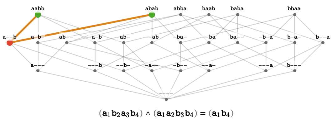
We can visualize this partial order for our example \( \regionalStates{\rewritingSystem{R}} \) via its Hasse diagram:
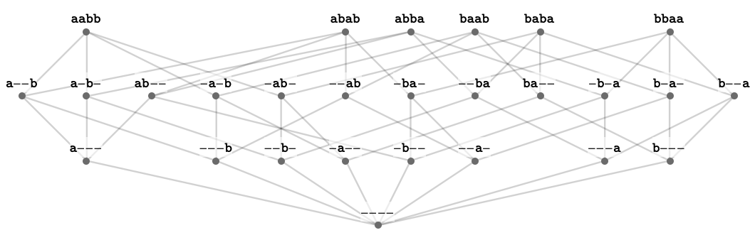
Notice that the global states \( \globalStatesSymbol \) correspond to the maximal elements of this partial order. The unique minimal element of the entire semilattice is the empty regional state \( \emptyRegionalState \syntaxEqualSymbol \wstring{\lstr{\texttt{----}}} \), which is less specific than any regional state. This element is written \( \semilatticeBottom \) in an order-theoretic context, and is called the bottom element.
Notice that the local states \( \localStatesSymbol \) correspond to the minimal non-bottom elements of this order (known as the atoms of the semilattice). We can also identify the local states by way of the covering relation: an element \( \posetElementSymbol{x} \) is said to cover and \( \posetElementSymbol{y} \) in a poset, written \( \posetElementSymbol{x}\posetCoversSymbol \posetElementSymbol{y} \), when both \( \posetElementSymbol{x}\posetGreaterSymbol \posetElementSymbol{y} \) and there does not exist another element \( \posetElementSymbol{z} \) such that \( \posetElementSymbol{x}\posetGreaterSymbol \posetElementSymbol{z}\posetGreaterSymbol \posetElementSymbol{y} \). Then the local states are those that cover the bottom element \( \semilatticeBottom \):
\[ \localStatesSymbol = \setConstructor{\regionalStateSymbol{R}}{\elemOf{\regionalStateSymbol{R}}{\regionalStatesSymbol },\regionalStateSymbol{R}\posetCoversSymbol \emptyRegionalState } \]Meet semilattice #
The set of regional states \( \regionalStatesSymbol \) has the additional order-theoretic structure of a meet semilattice. What is a meet semilattice? It is a partially ordered set \( \TuFo{\posetSymbol{X}, \posetLessEqualSymbol } \) with an additional binary operation called meet: \( \functionSignature{\function{\semilatticeMeetSymbol }}{\TuFo{\posetSymbol{X}, \posetSymbol{X}}}{\posetSymbol{X}} \) that takes a pair of elements to their greatest lower bound under the partial order \( \posetLessEqualSymbol \). In other words, the meet is defined to be the following operation:
\[ \meetSemilatticeElementSymbol{x}\semilatticeMeetSymbol \meetSemilatticeElementSymbol{y}\defEqualSymbol \indexMax{\suchThat{\meetSemilatticeElementSymbol{z}}{\meetSemilatticeElementSymbol{z}\posetLessEqualSymbol \meetSemilatticeElementSymbol{x},\meetSemilatticeElementSymbol{y}}}{\substack{\elemOf{\meetSemilatticeElementSymbol{z}}{\posetSymbol{X}}}}{} \]This function must be well-defined, that is, there must be a unique such maximal element for a poset to be a meet semilattice (in a total order, the maximum is always unique, but a set of elements of a poset that is not a total order can have several such maxima, which are necessarily pairwise incomparable).
In the case of regional states, the partial order is given by containment \( \regionalSubstateSymbol \), and the meet \( \regionalStateSymbol{R}\semilatticeMeetSymbol \regionalStateSymbol{S} \) of two regional states is simply the disjunction \( \regionalStateSymbol{R}\infixStateMeetSymbol \regionalStateSymbol{S} \) we have already defined, which satisfies the required property by definition.
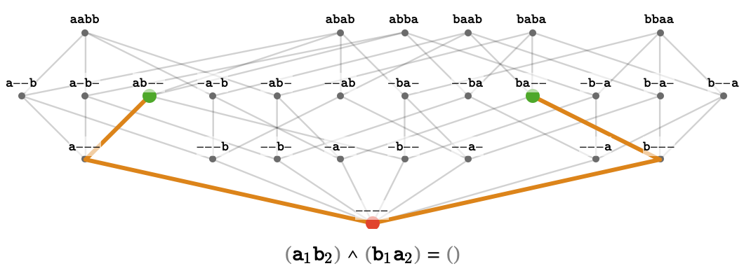
Illustration of meets #
Here we illustrate several meet operations in the regional state semilattice.
Relation between extent and specificity #
Phrased in terms of extent, then, we can have the following implication:
\[ \regionalStateSymbol{S}\regionalSubstateSymbol \regionalStateSymbol{R}\implies \stateExtent(\regionalStateSymbol{R}) \subseteq \stateExtent(\regionalStateSymbol{S}) \]In other words, if \( \regionalStateSymbol{R} \) is more specific than \( \regionalStateSymbol{S} \), the extent of \( \regionalStateSymbol{R} \) is a subset of the extent of \( \regionalStateSymbol{S} \). This makes sense: making a filter more specific will necessarily cause fewer global states to match it. This makes the function \( \stateExtent \) into a monotone function between the poset \( \TuFo{\regionalStatesSymbol , \regionalSubstateSymbol } \) of regional states and the poset \( \TuFo{\powerSet{\globalStatesSymbol }, \subseteq } \) of sets of global states.
Intent #
There is a natural "inverse" of the extent function, which we'll call intent. It maps a set of global states to a regional state that attempts to describe this set. The signature of \( \stateIntent \) is:
\[ \functionSignature{\stateIntent}{\powerSet{\globalStatesSymbol }}{\regionalStatesSymbol } \]Formally, it is defined to be the most specific regional state whose extent includes the input set of global states:
\[ \stateIntent(\setSymbol{G})\defEqualSymbol \indexMax{\suchThat{\regionalStateSymbol{R}}{\elemOf{\regionalStateSymbol{R}}{\regionalStatesSymbol },\stateExtent(\regionalStateSymbol{R}) \supseteq \setSymbol{G}}}{}{} \]The intent is bounded below by the disjunction of the input global states (when they are embedded into the corresponding regional states), since this disjunction matches all the input global states and so participates in the above maximization.
\[ \stateIntent(\setSymbol{G})\regionalSuperstateSymbol \stateMeet(\setConstructor{\function{ \iota }(\globalStateSymbol{g})}{\elemOf{\globalStateSymbol{g}}{\setSymbol{G}}}) = \stateCompose(\indexIntersection{\stateDecompose(\function{ \iota }(\globalStateSymbol{g}))}{\elemOf{\globalStateSymbol{g}}{\setSymbol{G}}}{}) \]In some cases, the intent is exactly the inverse of the extent. This is true whenever we apply intent to an set of global states that can be described exactly as the extent of some regional state:
\[ \forAllForm{\elemOf{\regionalStateSymbol{R}}{\regionalStatesSymbol }}{\stateIntent(\stateExtent(\regionalStateSymbol{R}))\identicallyEqualSymbol \regionalStateSymbol{R}} \]As an example, consider the set \( \setSymbol{G} = \SeFo{\qstring{\lstr{\texttt{aabb}}}, \qstring{\lstr{\texttt{baba}}}} \). The intent of \( \setSymbol{G} \) is the regional state \( \wstring{\lstr{\texttt{-ab-}}} \), because specifying any characters beyond the middle two will prevent one or both of the elements of \( \setSymbol{G} \) from matching. Moreover, this regional state specifies exactly one \( \lchar{\texttt{a}} \) and one \( \lchar{\texttt{b}} \), and so there are only two ways of fixing the unspecified string positions, meaning the regional state has exactly the extent \( \setSymbol{G} \). Summarizing this situation:
\[ \begin{aligned} \setSymbol{G}&= \SeFo{\qstring{\lstr{\texttt{aabb}}}, \qstring{\lstr{\texttt{baba}}}}\\ \stateIntent(\setSymbol{G})&= \wstring{\lstr{\texttt{-ab-}}}\\[1em] \stateExtent(\stateIntent(\setSymbol{G}))&= \stateExtent(\wstring{\lstr{\texttt{-ab-}}})\\ &= \SeFo{\qstring{\lstr{\texttt{aabb}}}, \qstring{\lstr{\texttt{baba}}}}\\ &= \setSymbol{G}\end{aligned} \]However, not all sets of global states are of this form. In particular, if there is pair of incompatible states within a pair of global states in the input set, this forces a blind spot in any regional state whose extent includes this pair of global states, and this blind spot can let other global states through that are not in the input set.
A simple example of this situation for \( \rewritingSystem{R_2} \) occurs for the set \( \setSymbol{G} = \SeFo{\qstring{\lstr{\texttt{aabb}}}, \qstring{\lstr{\texttt{bbaa}}}} \). This two global states are maximally incompatible, in that the only regional state that matches both of them is the empty regional state. This is because the melt of these two global states has zero intersection: they disagree in all string positions. Hence, the intent of \( \setSymbol{G} \) is \( \emptyRegionalState \syntaxEqualSymbol \wstring{\lstr{\texttt{----}}} \), which in turn matches all global states:
\[ \begin{aligned} \setSymbol{G}&= \SeFo{\qstring{\lstr{\texttt{aabb}}}, \qstring{\lstr{\texttt{bbaa}}}}\\ \stateIntent(\setSymbol{G})&= \wstring{\lstr{\texttt{----}}}\\[1em] \stateExtent(\stateIntent(\setSymbol{G}))&= \stateExtent(\wstring{\lstr{\texttt{----}}})\\ &= \globalStatesSymbol \end{aligned} \]Notice that while we do not have equality between \( \setSymbol{G} \) and \( \stateExtent(\stateIntent(\setSymbol{G})) \) for some arbitrary set \( \elemOf{\setSymbol{G}}{\powerSet{\globalStatesSymbol }} \), they are at least comparable:
\[ \setSymbol{G} \subseteq \stateExtent(\stateIntent(\setSymbol{G})) \]In words: taking the extent of the intent of a set of global states can either keep the set the same or enlarge it with novel states.
Galois connection #

Diagram #
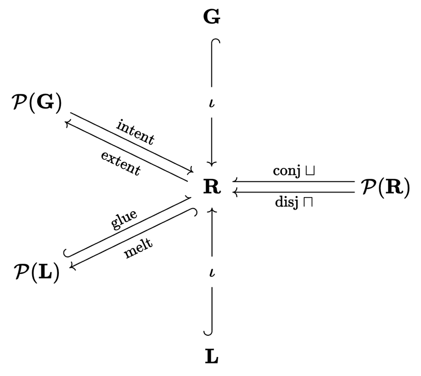
This diagram illustrates the functions between local, regional, and global states. A half-arrowhead indicates a partial function. We enumerate these functions here:
| z | z |
|---|---|
| \( \functionSignature{\function{ \iota }}{\localStatesSymbol }{\regionalStatesSymbol } \) | embeds local state into atomic regional state |
| \( \functionSignature{\function{ \iota }}{\globalStatesSymbol }{\regionalStatesSymbol } \) | embeds global state into maximal regional state |
| \( \partialFunctionSignature{\stateCompose}{\powerSet{\localStatesSymbol }}{\regionalStatesSymbol } \) | glues set of local states into regional state |
| \( \functionSignature{\stateDecompose}{\regionalStatesSymbol }{\powerSet{\localStatesSymbol }} \) | melts regional state into set of compatible local states |
| \( \functionSignature{\stateExtent}{\powerSet{\globalStatesSymbol }}{\regionalStatesSymbol } \) | gives set of global states matching regional state |
| \( \functionSignature{\stateIntent}{\regionalStatesSymbol }{\powerSet{\globalStatesSymbol }} \) | gives most specific regional state that matches set of global states |
| \( \partialFunctionSignature{\stateJoin}{\powerSet{\regionalStatesSymbol }}{\regionalStatesSymbol } \) | gives least specific regional state more specific than set of regional states |
| \( \functionSignature{\stateMeet}{\powerSet{\regionalStatesSymbol }}{\regionalStatesSymbol } \) | gives most specific regional state less specific than set of regional states |
Rewrite rules as schemas #
Generalizing linear algebra with atrices #
Petri nets #
Causal bigraph and causal hypergraph #
Compilation #
Rewriting systems to hypergraph rewriting systems #
Hypergraph rewriting systems to petri nets #